Election Forecasting (Putting It All Together)

POLS 3220: How to Predict the Future

dn = (x, m, s) => Math.exp(-0.5 * ((x - m) / s) ** 2) / (s * Math.sqrt(2 * Math.PI))
grid = d3.range(-60, 60.001, 0.1)
col = ({prior: "#4a7ab0", poll: "#d1495b", post: "#6a3d9a", actual: "#222"})
fmt = (x) => (x > 0 ? "D+" : x < 0 ? "R+" : "") + Math.abs(x).toFixed(1)

Today’s Agenda

• Over the past two weeks, we’ve approached election forecasting from two perspectives:

  1. The Polls: unbiased, but much noisier than classical theory predicts.

  2. The Fundamentals: political and economic indicators historically correlated with election outcomes.

• Today, we combine them into a single forecasting model for US Senate elections.

• To do so, we’ll need the help of an old friend: Bayes Rule.

The Polls

Recap: Polling Averages

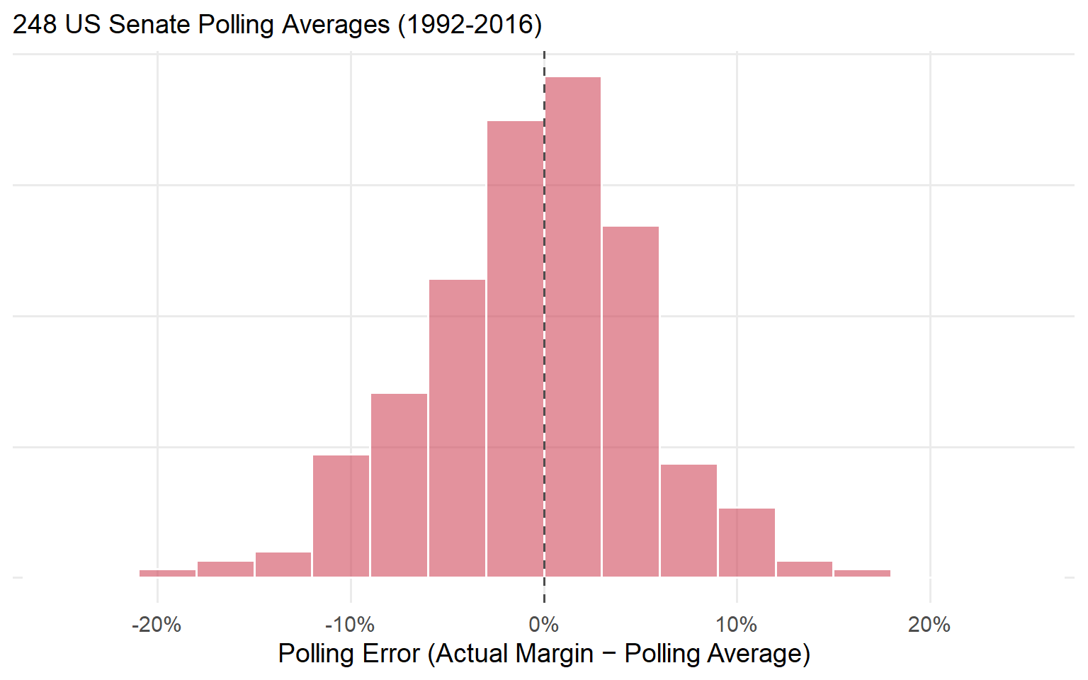
Recap: Polling Averages

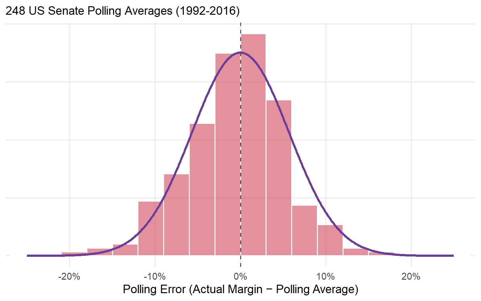
Polling averages are unbiased, with errors that fall on a bell curve (SD = 5.7 points).

Within 1 / 2 / 3 SD: 71% / 95% / 99% (bell curve: 68 / 95 / 99.7). Net bias -0.6 points.

Sampling theory alone predicts an SD of about 1.4 points (pooling everyone surveyed in a race’s polls), so real error is about 4x wider: non-response, late deciders, likely-voter screens, pollsters making correlated mistakes.

The Fundamentals

Recap: The Fundamentals

• Last time, we built a fundamentals model of presidential elections using June presidential approval and Q2 GDP growth.

• That model had an average error of about 3.6 percentage points.

• Can we do the same thing for Senate elections?

• The problem here is a lack of good data: there’s no “Senator approval rating” or “state GDP growth” dataset going back decades.

• But there are still some useful predictors:

  • The Cook Political Report’s Partisan Voting Index (PVI): how much more Democratic or Republican a state votes than the country as a whole.

  • Whether each Senate candidate has previous political experience (Carson et al. 2010).

Senate Fundamentals

Fitting a linear model to 397 Senate elections (1992-2016) yields this equation:

\[ \begin{aligned} \text{Democratic Margin} = -0.1 & + 1.2 \times \text{ PVI } \\ & + 18.0 \times \text{ Democrat Experienced } \\ & - 15.3 \times \text{ Republican Experienced } \end{aligned} \]

• Every point of PVI is worth about 1.2 points of vote margin.

• An experienced Democrat gains about 18 points; an experienced Republican, about 15 points.

How Predictive Are The Fundamentals?

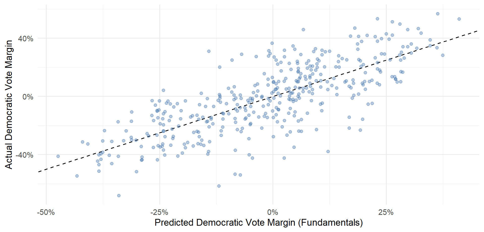
How Predictive Are The Fundamentals?

Model	Elections	Average Error	Brier
President (June Approval + Q2 GDP)	11	3.6 pts	0.099
Senate (PVI + Experience)	397	12.2 pts	0.129

• The Senate fundamentals model’s average error is about 12 points.

• That’s about 3 times worse than the presidential model, and about 3 times worse than the polling averages (4.3 points).

• Discuss: Why might Senate fundamentals be so much weaker than presidential fundamentals?

Candidates vary much more (scandals, quality, money); local issues; no good race-specific economic or approval data; incumbency is a big missing variable here.

Polls + Fundamentals

Recap: Bayes Rule

\[ \text{Posterior Odds} = \text{Prior Odds} \times \text{Strength of Evidence} \]

• Start with a prior: what you believed before seeing the evidence.

• Ask how much more likely the evidence is under one possibility than another: the strength of evidence.

• Multiply to get your posterior: what you believe after seeing the evidence.

The Prior

West Virginia, 2018. Before looking at any polls, the fundamentals predict R+13.5.

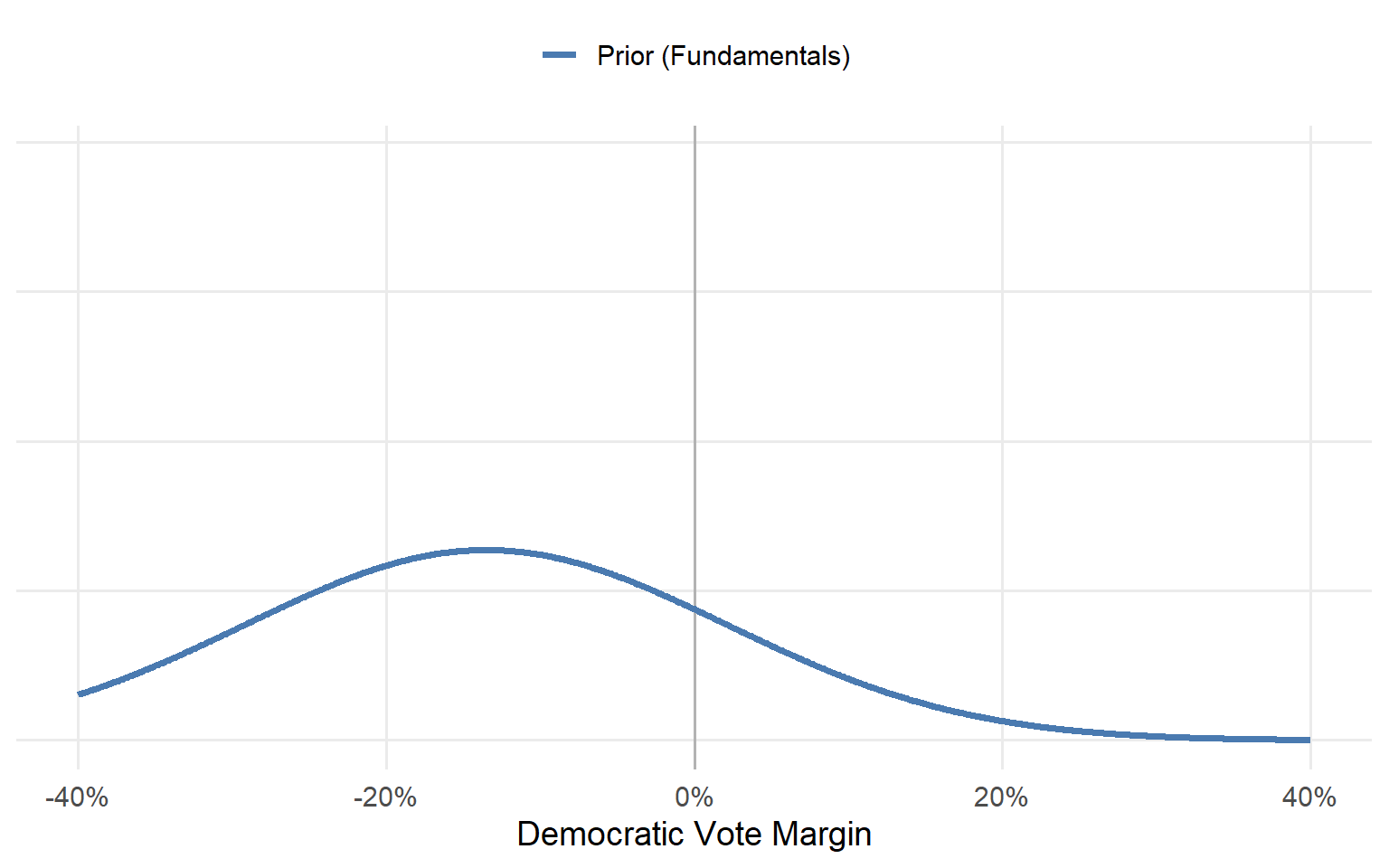
The Evidence

The polling average in the final month was D+9.2.

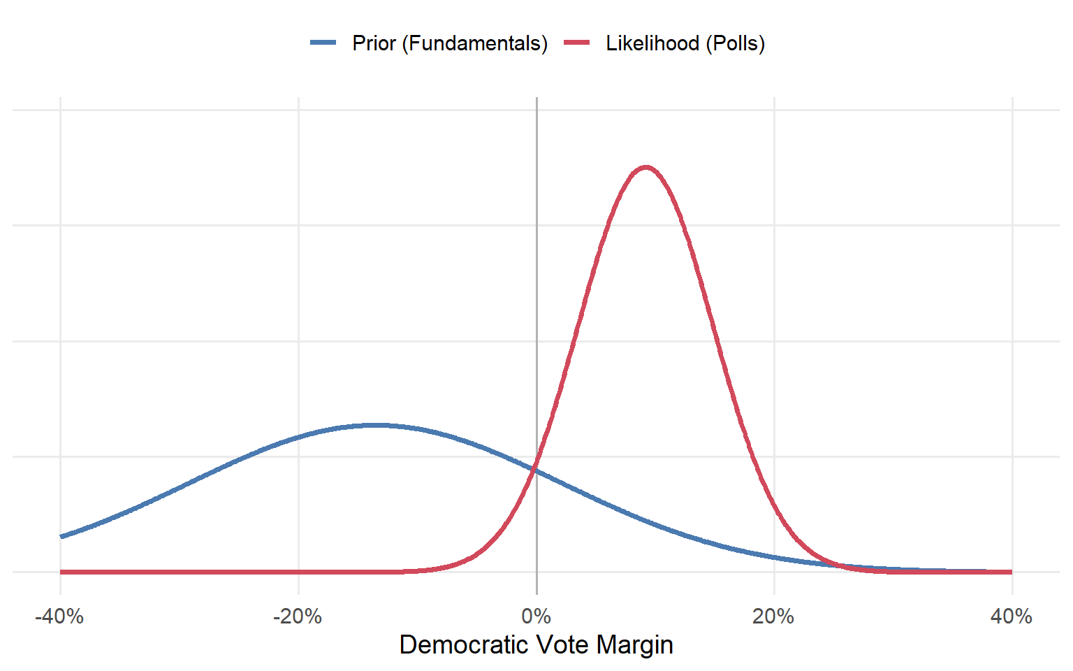
Posterior = Prior × Likelihood

// R's NA arrives as the string "NA", so keep only races with a numeric polling average
viewof race = Inputs.select(transpose(races18).filter(d => typeof d.poll === "number").map(d => d.raceid).sort(),
  {value: "West Virginia-2018", label: "2018 race"})

{
  const r = transpose(races18).find(d => d.raceid === race);
  const pr = grid.map(x => dn(x, r.prior, consts.sd_prior));
  const lk = grid.map(x => dn(r.poll, x, consts.sd_poll));      // likelihood of the observed polls
  const prod = pr.map((p, i) => p * lk[i]);
  const Z = d3.sum(prod) * 0.1;
  const post = prod.map(p => p / Z);
  const pm = d3.sum(grid.map((x, i) => x * post[i] * 0.1));
  const pwin = d3.sum(grid.map((x, i) => (x > 0 ? post[i] * 0.1 : 0)));
  const rows = (arr, key) => grid.map((x, i) => ({x, y: arr[i], key}));
  const data = [...rows(pr, "Prior (fundamentals)"), ...rows(lk, "Likelihood (polls)"), ...rows(post, "Posterior")];
  // one row per margin for the hover readout (every 0.5 pts, within the visible range)
  const hover = grid.map((x, i) => ({x, pr: pr[i], lk: lk[i], prod: prod[i], post: post[i]}))
    .filter((d, i) => i % 5 === 0 && Math.abs(d.x) <= 40);
  const at = (key) => Plot.pointerX({x: "x", y: key, fill: col[{pr: "prior", lk: "poll", post: "post"}[key]], r: 5});
  return html`<div>${Plot.plot({
    width: 900, height: 400, style: {fontSize: "15px"}, marginBottom: 50,
    x: {label: "Dem margin (pts)", labelAnchor: "center", labelOffset: 42, domain: [-40, 40]},
    y: {label: null, ticks: []},
    color: {domain: ["Prior (fundamentals)", "Likelihood (polls)", "Posterior"],
            range: [col.prior, col.poll, col.post], legend: true},
    marks: [
      Plot.areaY(rows(post, "Posterior"), {x: "x", y: "y", fill: col.post, fillOpacity: 0.15}),
      Plot.line(data, {x: "x", y: "y", stroke: "key", strokeWidth: 2.5}),
      Plot.ruleX([0], {stroke: "#999"}),
      // hover: rule + a dot on each curve + the multiplication
      Plot.ruleX(hover, Plot.pointerX({x: "x", stroke: "orange", strokeWidth: 1.5})),
      Plot.dot(hover, at("pr")), Plot.dot(hover, at("lk")), Plot.dot(hover, at("post")),
      Plot.tip(hover, Plot.pointerX({x: "x", y: d => Math.max(d.pr, d.lk, d.post), fontSize: 14,
        title: d => `At ${fmt(d.x)}\nprior ${d.pr.toFixed(4)} × likelihood ${d.lk.toFixed(4)}\n= ${d.prod.toExponential(2)}\n→ posterior ${d.post.toFixed(4)} (rescaled)`}))
    ]
  })}
  <p style="font-size: 0.72em; margin: 0">
  Prior ${fmt(r.prior)} · Polls ${fmt(r.poll)} (${r.num_polls} polls) · <b>Posterior ${fmt(pm)}</b>
  · P(Democrat wins) = <b>${(pwin * 100).toFixed(0)}%</b></p></div>`;
}

If anyone asks why the posterior hugs the polls:

• Where the polls’ curve is tall, the fundamentals’ curve is nearly flat. Multiplying by something nearly flat barely changes the shape.
• When both curves are bell curves, the posterior is a weighted average: Posterior = w × Fundamentals + (1 − w) × Polls.
• Each source’s weight depends on its precision, one over its variance (1/SD^2). Fundamentals: 1/15.7^2. Polls: 1/5.7^2. So the fundamentals get 12% of the weight and the polls get 88%.
• The posterior is also more precise than either source alone: SD = 5.3 points (vs. 15.7 and 5.7).

Derivation. Write the prior as N(m1, s1^2) (fundamentals) and the likelihood as N(m2, s2^2) (polls). Their product, as a function of the true margin x, is proportional to

exp( -(x - m1)^2 / (2 s1^2) - (x - m2)^2 / (2 s2^2) )

The exponent is a quadratic in x. Expand and collect terms: the x^2 coefficient is -(1/s1^2 + 1/s2^2)/2 and the x coefficient is (m1/s1^2 + m2/s2^2). Completing the square gives another bell curve with

precision 1/s^2 = 1/s1^2 + 1/s2^2 (precisions add)

mean m = (m1/s1^2 + m2/s2^2) / (1/s1^2 + 1/s2^2) = w m1 + (1 - w) m2, where w = (1/s1^2) / (1/s1^2 + 1/s2^2).

Here: 1/15.7^2 = 0.0041 and 1/5.7^2 = 0.0309, so w = 0.117.

The Combined Model

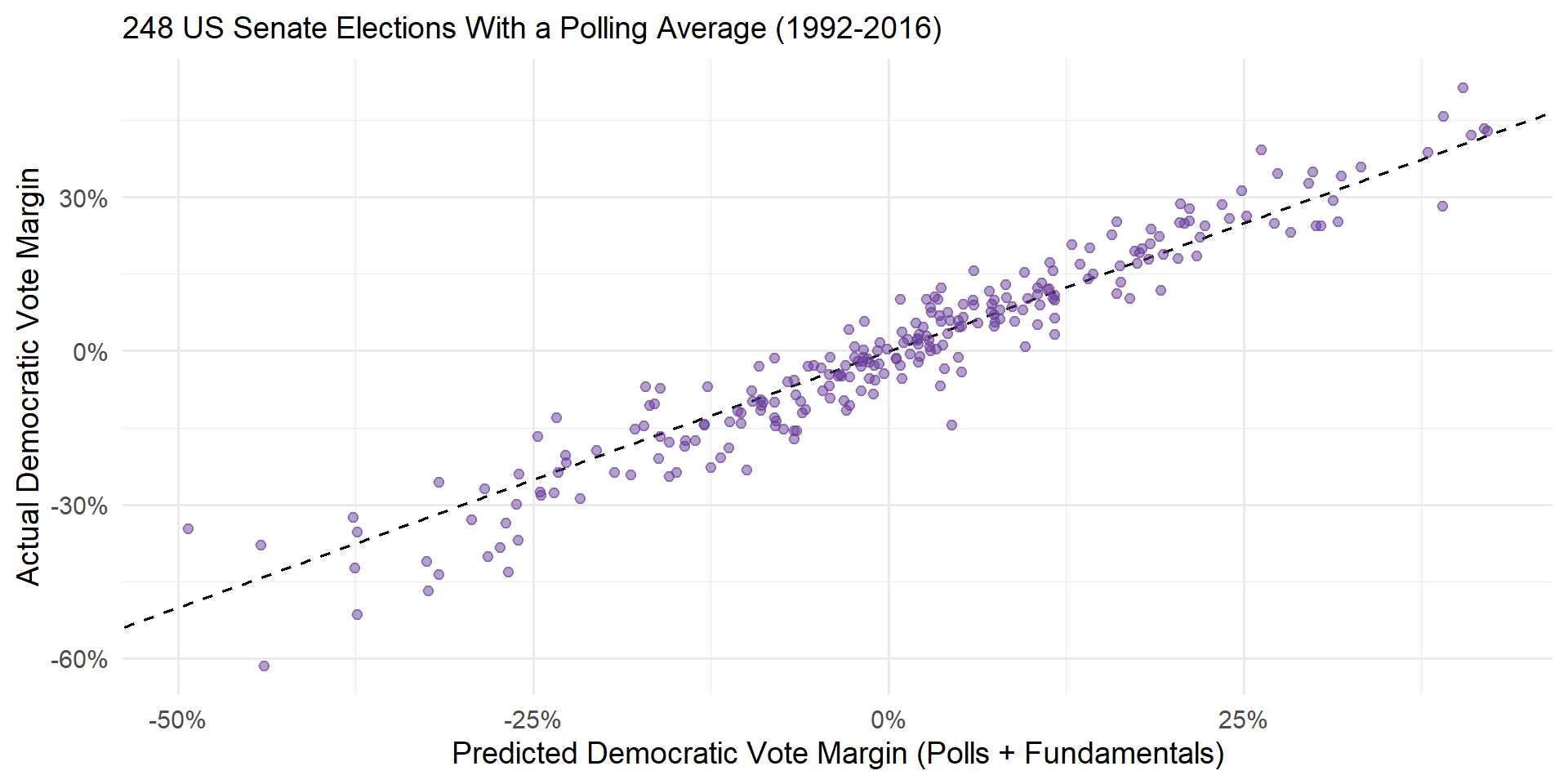
The Combined Model

• The combined model has an average error of 4.2 percentage points.

• It correctly calls the winner in 92.3% of elections from 1992-2016.

• But the true test of a model is whether it can accurately forecast out-of-sample.

  • The model was fit using 1992-2016 election data. Can the same model accurately predict election outcomes in 2018?

2018 Forecasts

viewof show = Inputs.checkbox(["Fundamentals", "Polls", "Posterior ± 95%", "Actual"],
  {value: ["Posterior ± 95%"], label: "Show"})

{
  const r = transpose(races18).map(d => ({...d, race: d.raceid.replace("-2018", "")}))
    .sort((a, b) => b.post - a.post);
  const has = (k) => show.includes(k);
  return Plot.plot({
    width: 900, height: 560, style: {fontSize: "14px"}, marginLeft: 120, marginBottom: 45,
    x: {label: "Predicted Democratic vote margin (pts)", labelAnchor: "center", labelOffset: 38,
        domain: [-70, 70], grid: true},
    y: {label: null, domain: r.map(d => d.race)},
    marks: [
      Plot.ruleX([0], {strokeDasharray: "4,4"}),
      has("Posterior ± 95%") ? Plot.ruleY(r, {y: "race", x1: d => d.post - 1.96 * d.post_sd,
        x2: d => d.post + 1.96 * d.post_sd, stroke: col.post, strokeOpacity: 0.35, strokeWidth: 5}) : null,
      has("Fundamentals") ? Plot.dot(r, {y: "race", x: "prior", stroke: col.prior, strokeWidth: 2, r: 4.5}) : null,
      has("Polls") ? Plot.dot(r.filter(d => typeof d.poll === "number"), {y: "race", x: "poll", fill: col.poll,
        symbol: "diamond", r: 5}) : null,
      has("Posterior ± 95%") ? Plot.dot(r, {y: "race", x: "post", fill: col.post, r: 4.5}) : null,
      has("Actual") ? Plot.dot(r, {y: "race", x: "actual", stroke: col.actual, symbol: "times", r: 6, strokeWidth: 2.5}) : null,
      Plot.tip(r, Plot.pointerY({y: "race", x: "post", fontSize: 14, title: d =>
        `${d.raceid}\nfundamentals ${fmt(d.prior)}\npolls ${typeof d.poll === "number" ? fmt(d.poll) + " (" + d.num_polls + " polls)" : "none"}\nposterior ${fmt(d.post)}\nactual ${fmt(d.actual)}`}))
    ]
  });
}

Out-of-Sample Prediction

• The polls + fundamentals model correctly predicted all but two of the 2018 Senate elections, with an average error of 3.1 percentage points.

• By comparison, if you had been looking at the polls alone, you would have incorrectly called three elections.

  • In Missouri 2018, the polls narrowly favored the Democratic incumbent, but the fundamentals were skeptical.

Takeaways

• It’s somewhat surprising that combining two noisy predictors (polls: 3.6% error, fundamentals: 7.3% error) yields a pretty good model (polls + fundamentals: 3.1% error)!

• But it follows the basic logic of the wisdom of crowds and Bayesian updating.

• Both polls and fundamentals provide an imperfect glimpse at the state of a race.

• Combining the two perspectives yields a better forecast than either alone (Chen et al. 2023).

References

Carson, Jamie, Gregory Koger, Matthew J. Lebo, Jamie L, and Matthew J. Lebo. 2010. “The Electoral Costs of Party Loyalty in Congress.” American Journal of Political Science, 598616.

Chen, Yehu, Roman Garnett, and Jacob M. Montgomery. 2023. “Polls, Context, and Time: A Dynamic Hierarchical Bayesian Forecasting Model for US Senate Elections.” Political Analysis 31 (1): 113–33. https://doi.org/10.1017/pan.2021.42.