Linear Models
POLS 3220: How to Predict the Future
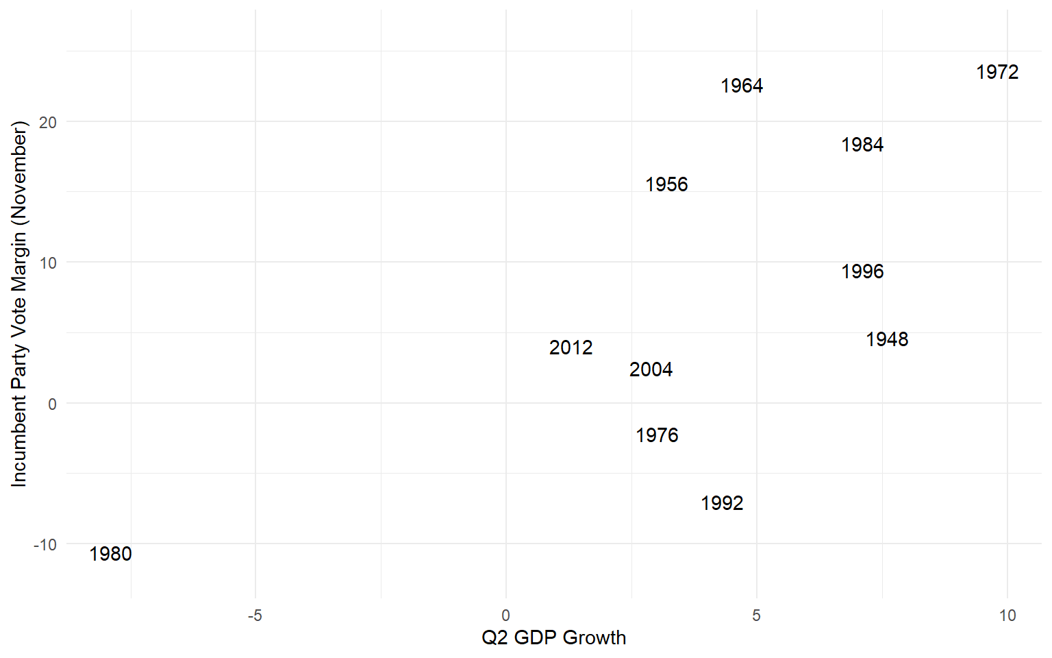
Machine Learning
Machine Learning

Machine Learning
Presidential Election Forecast
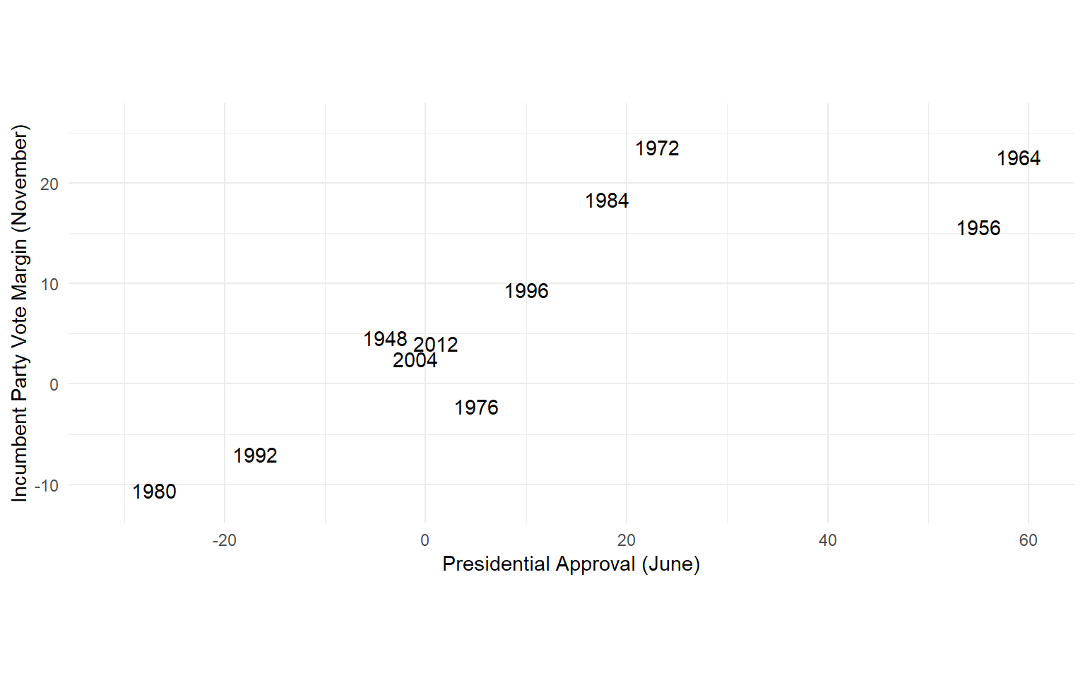
Presidential Election Forecast
Presidential Election Forecast
Presidential Election Forecast
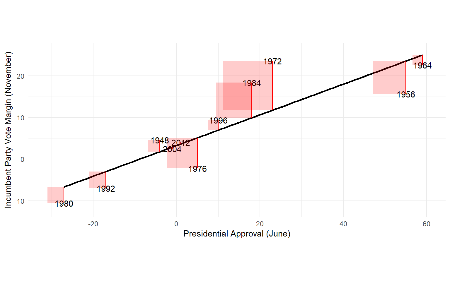
Presidential Election Forecast
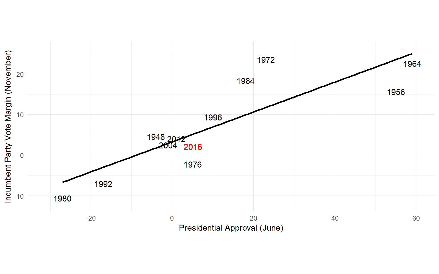
Presidential Election Forecast
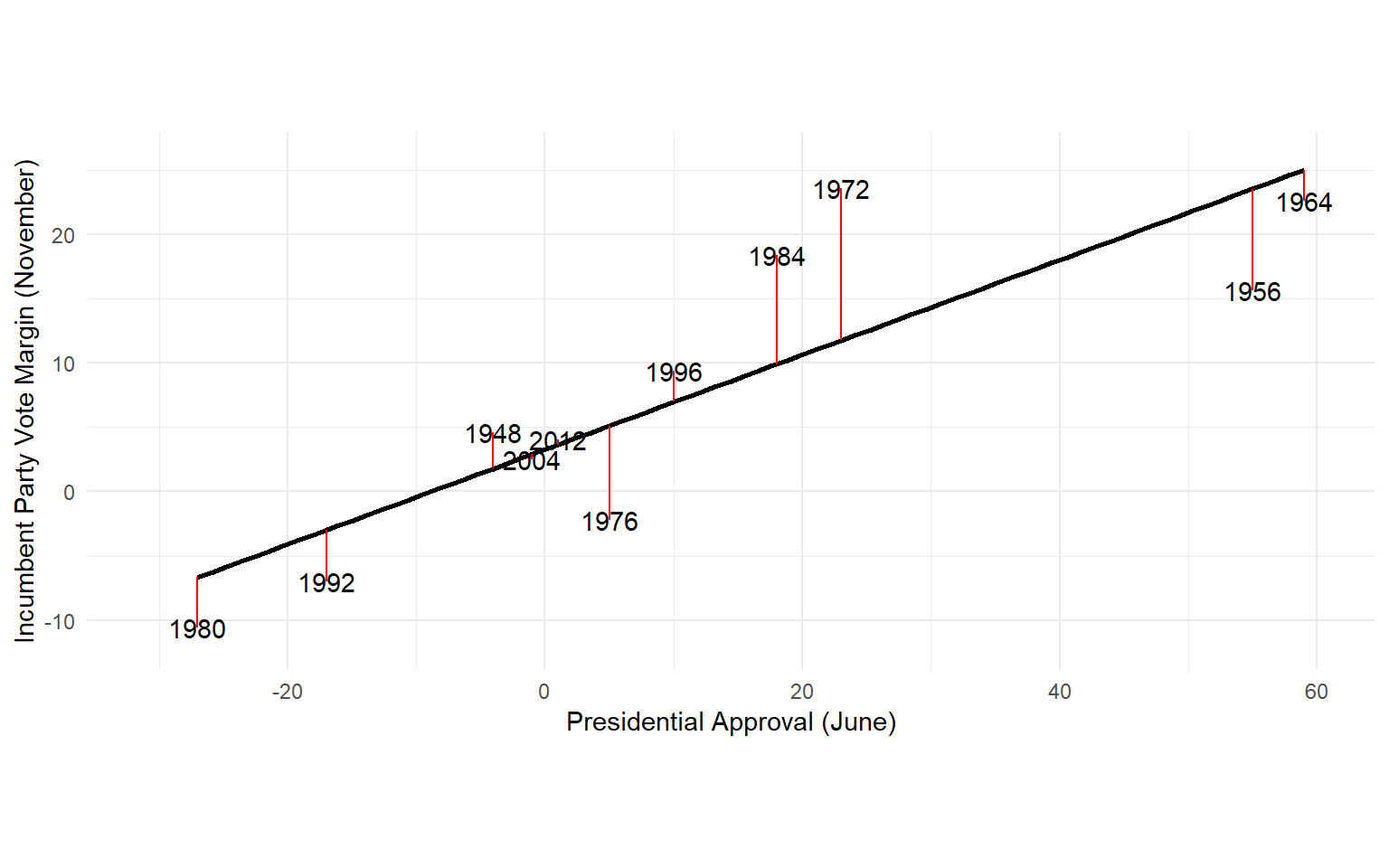
The average forecast error is 4.7 percentage points.
And we have some particularly large errors in 1972 (11.9 points) and 1984 (8.5 points).
Maybe we’d do better if we added more predictor variables to the model?

Presidential Election Forecast
Danger 1: Nonlinearity
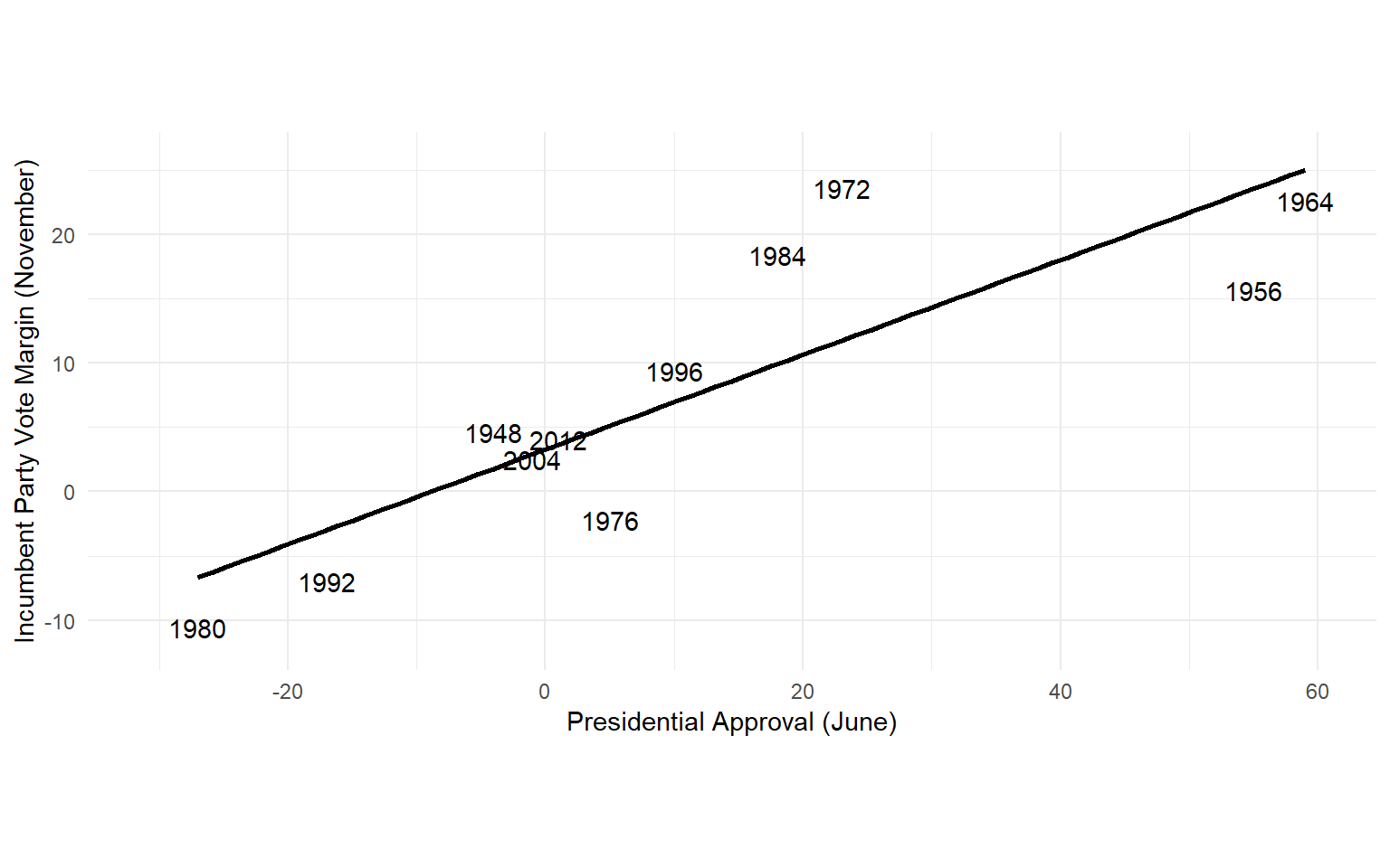
The linear model faithfully gives you the line of best fit…
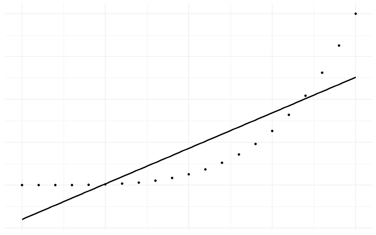
…even when a straight line is a terrible model!
- Diagnostic: are there patterns in the errors?
Danger 2: Extrapolation
- Be cautious of making predictions with a linear model if the current situation lies far outside the historical data.
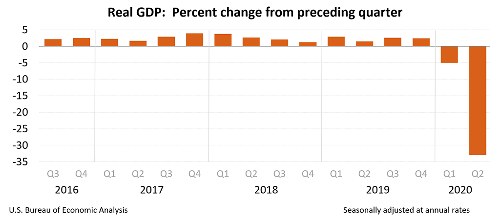
- Plugging these numbers into our model would predict the incumbent losing by 35.2 percentage points! (Actual margin was -4.5 points).