Long Tails
POLS 3220: How to Predict the Future
Warmup
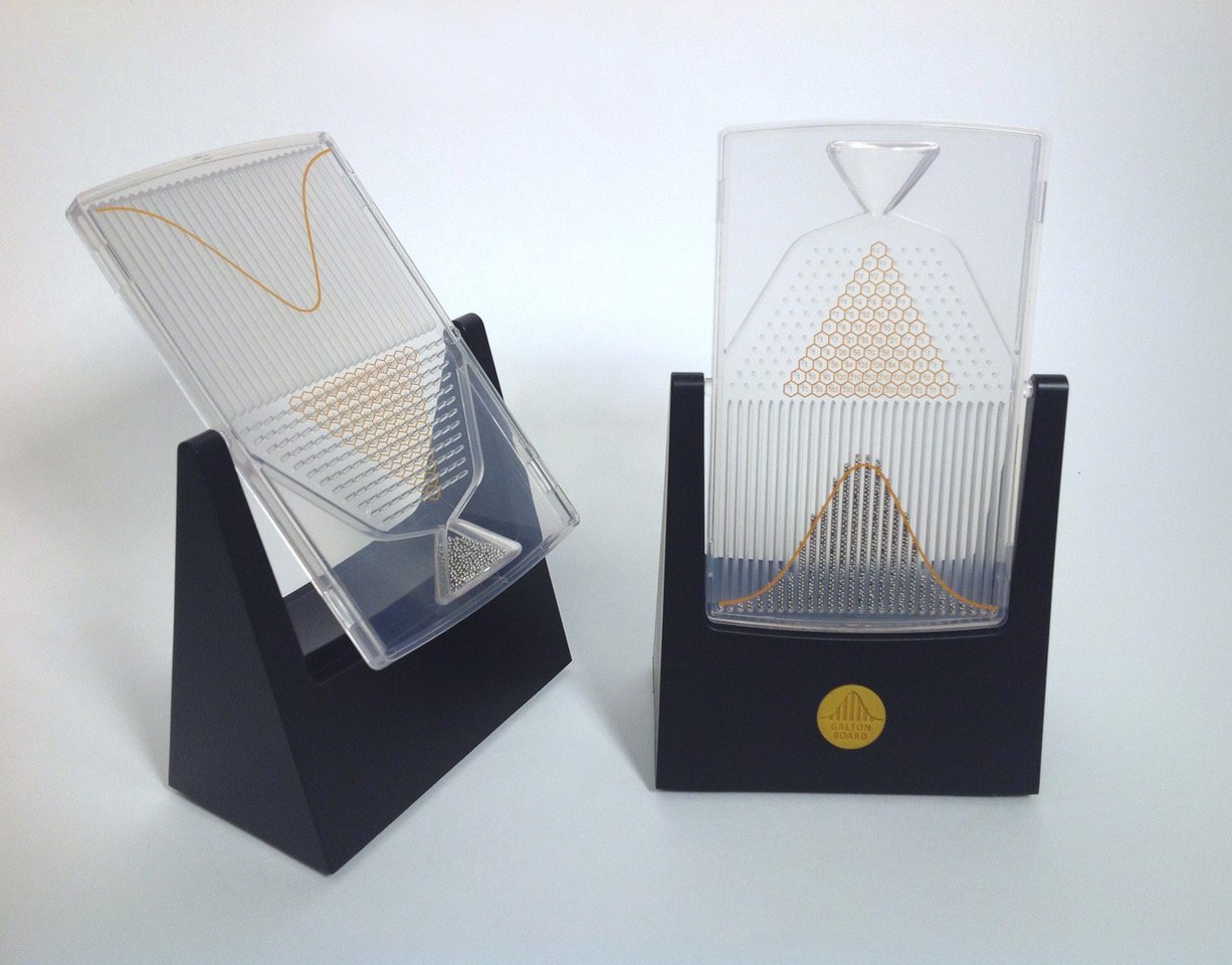
Using the definition of the Central Limit Theorem, explain why the Galton Board produces a bell curve shape.
Bell Curves Have Low Tail Risk
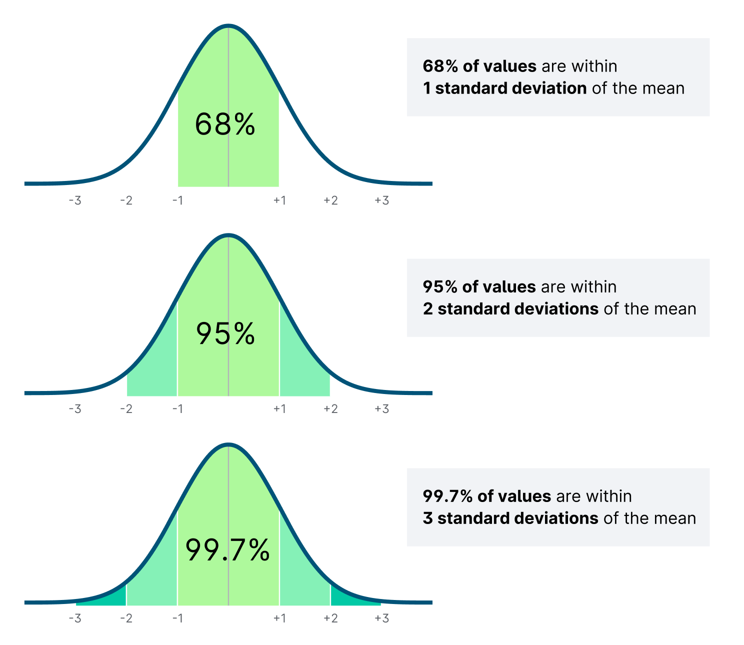
- Standard deviation \((\sigma)\) is a measure of the spread of the distribution. It measures how far, on average, observations lie from their expected value.
- A “2 sigma” event should happen only 5% of the time.
- A “3 sigma” event should happen only 0.3% of the time.
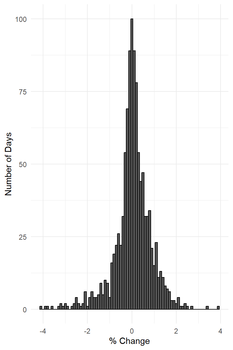
Financial Markets Example
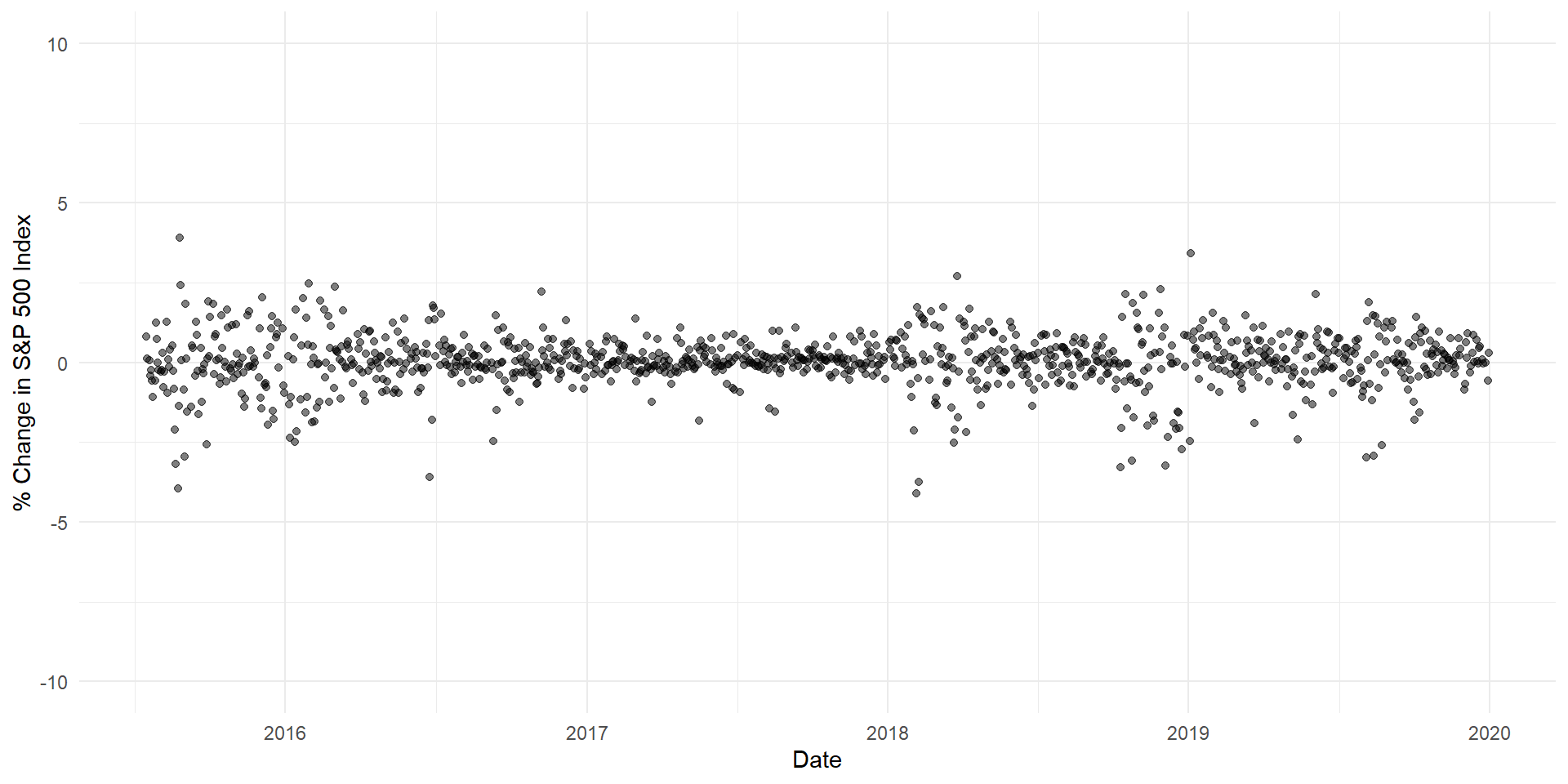
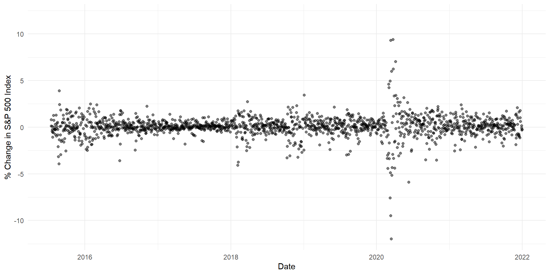
So what’s the problem?
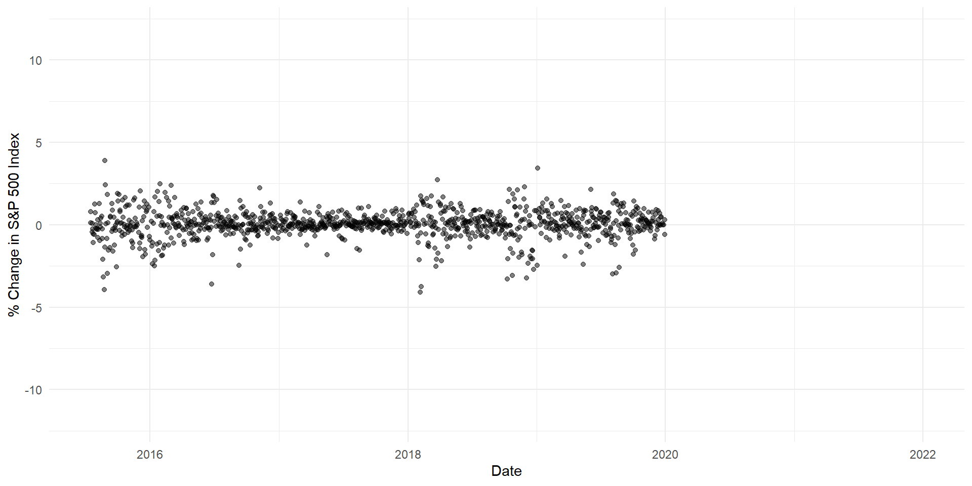
So what’s the problem?
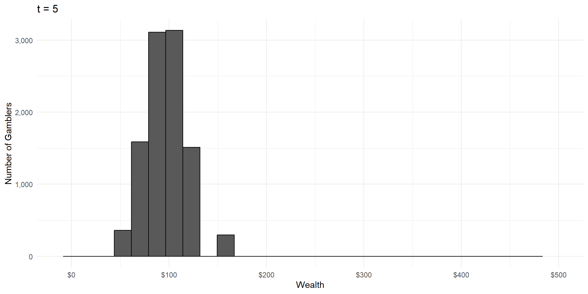
Violation 1: Multiplicative Processes
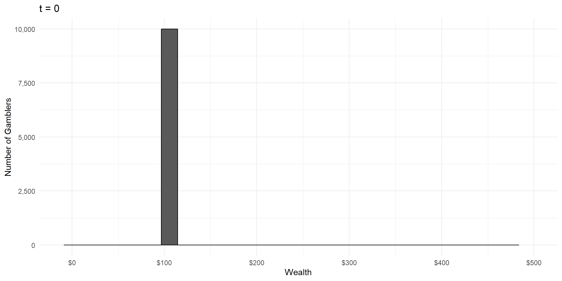
Violation 1: Multiplicative Processes
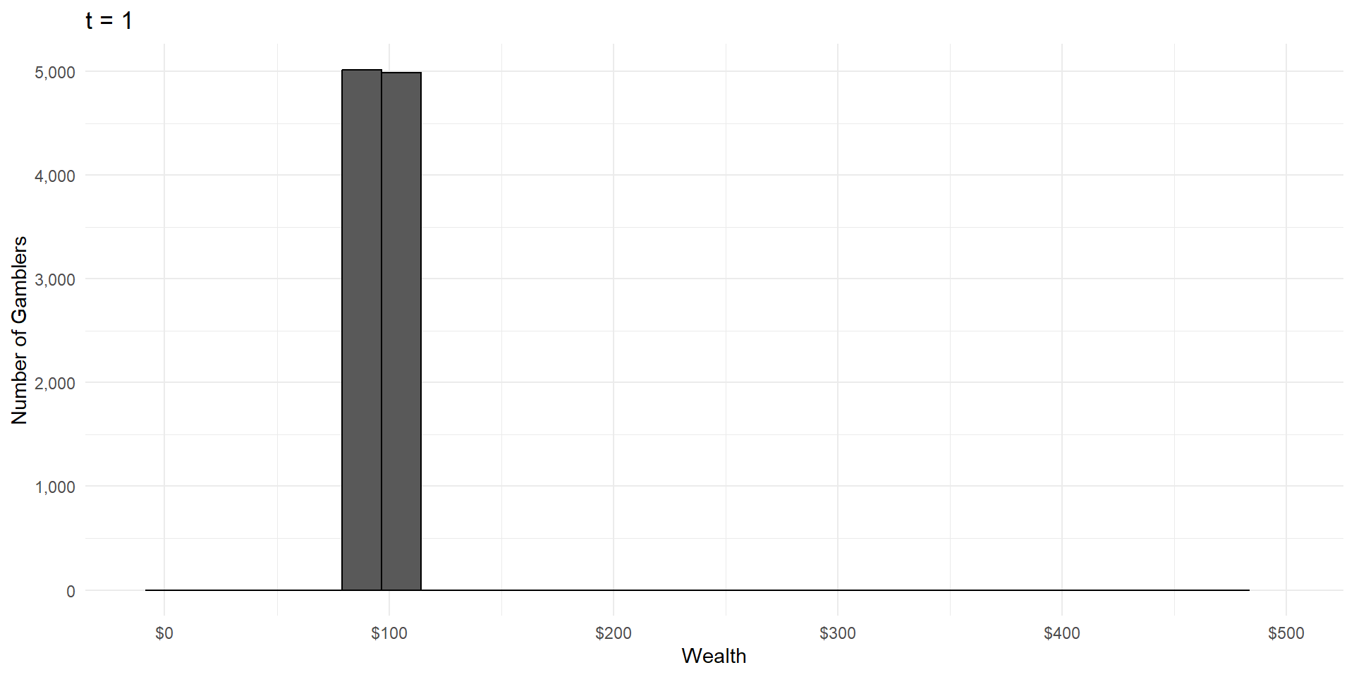
Violation 1: Multiplicative Processes
Violation 1: Multiplicative Processes
Violation 1: Multiplicative Processes
Violation 1: Multiplicative Processes
Violation 1: Multiplicative Processes
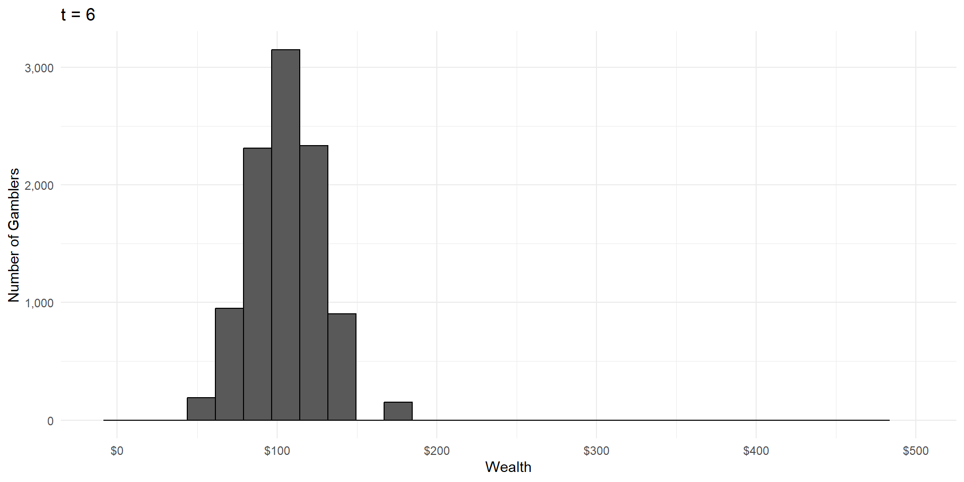
Violation 1: Multiplicative Processes
Violation 1: Multiplicative Processes

Violation 1: Multiplicative Processes
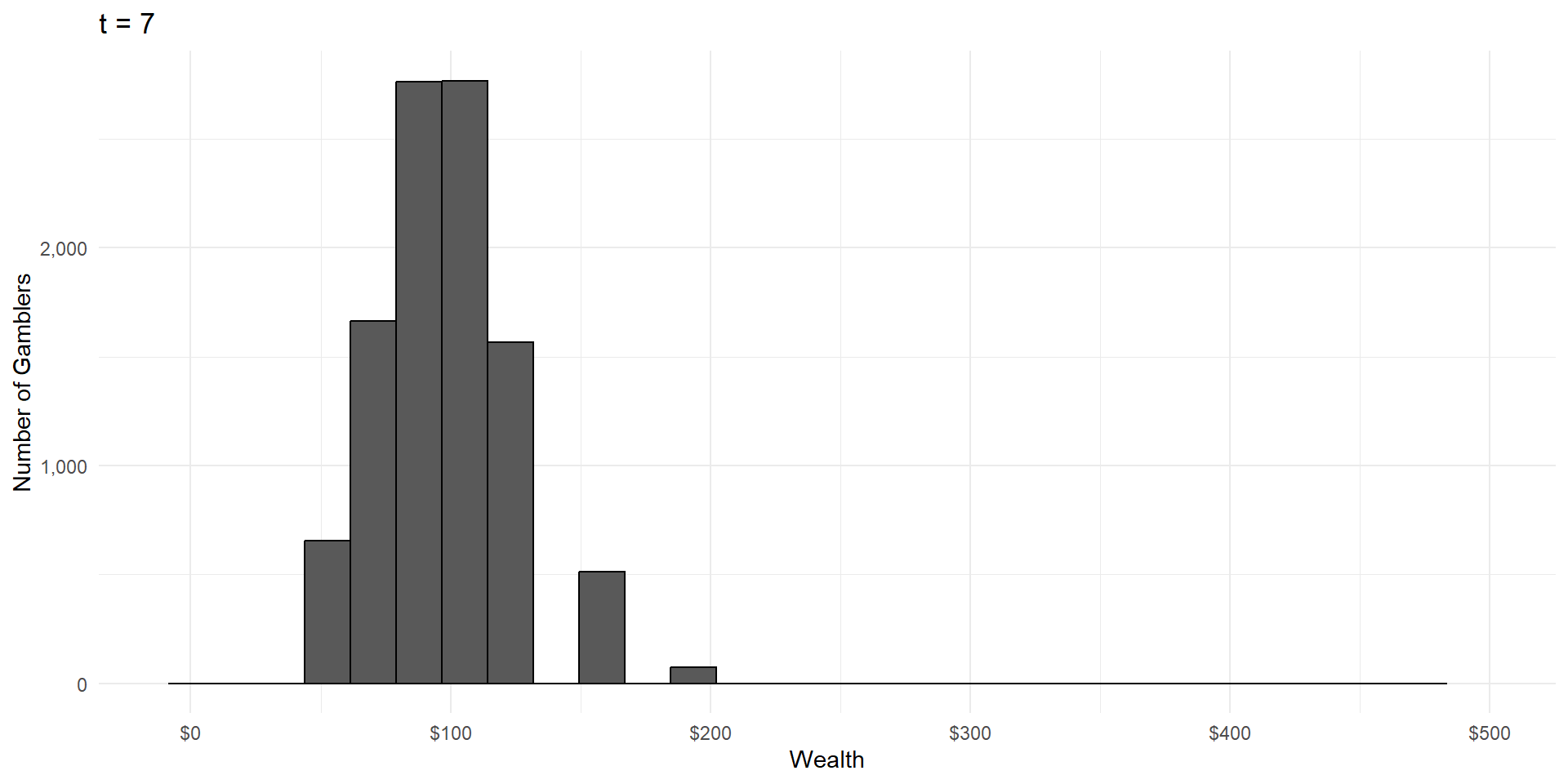
Violation 1: Multiplicative Processes
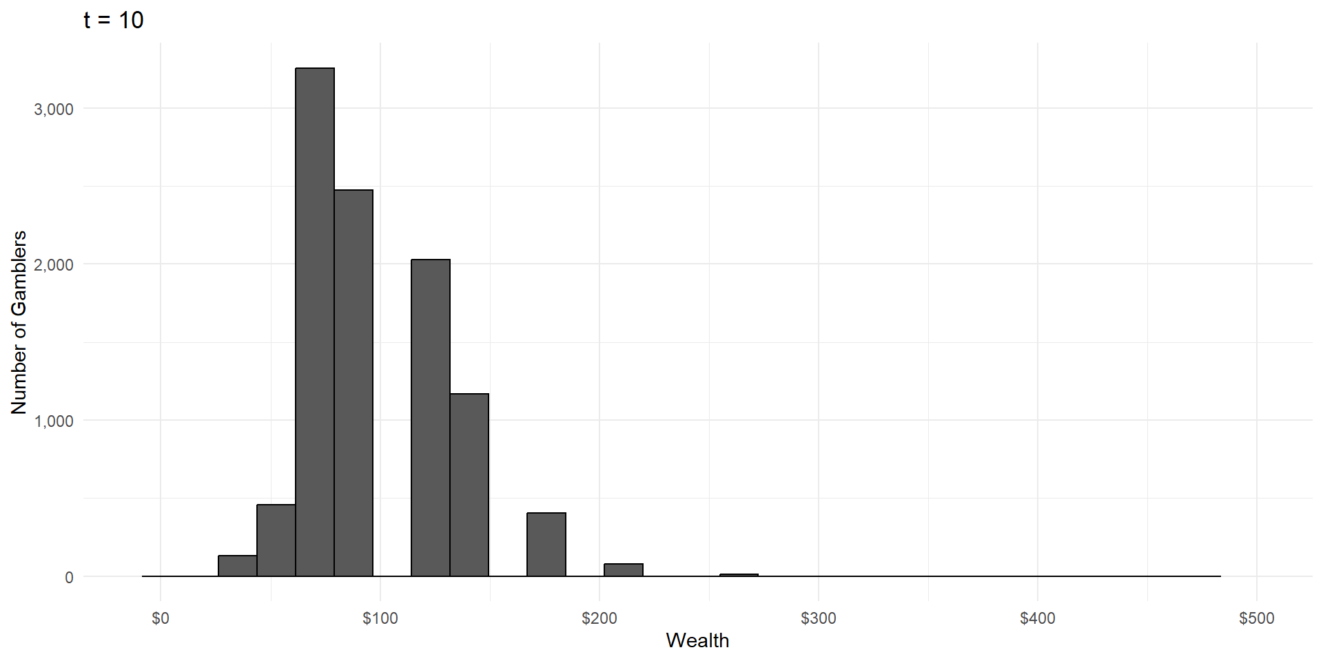
Violation 1: Multiplicative Processes
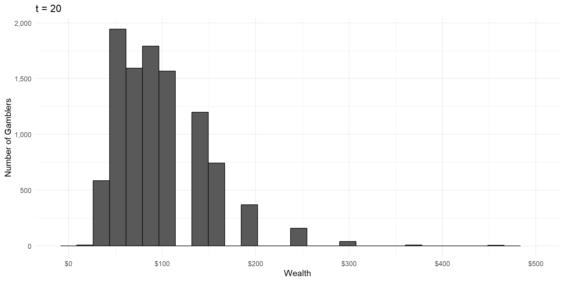
Violation 1: Multiplicative Processes
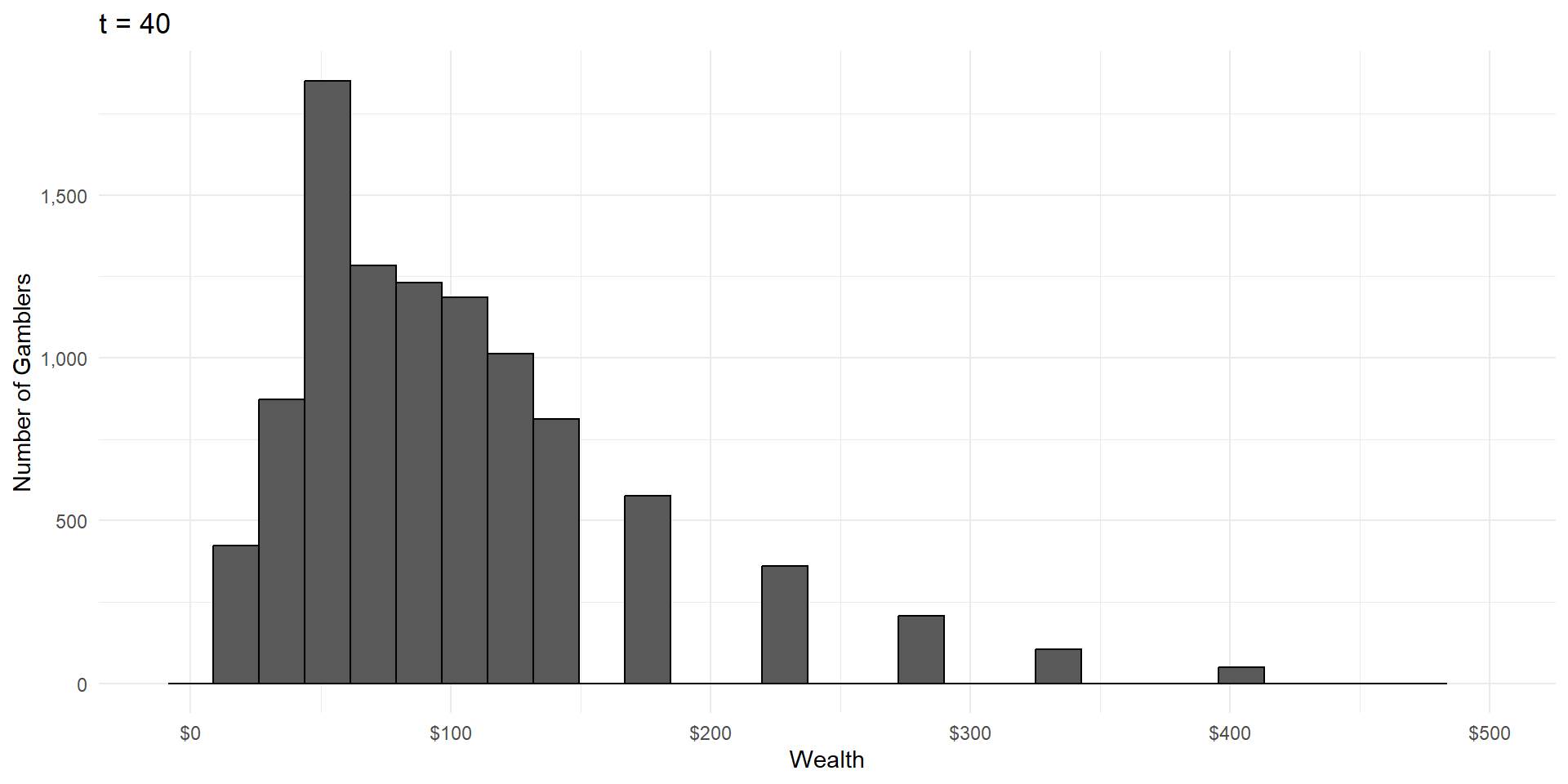
Violation 1: Multiplicative Processes
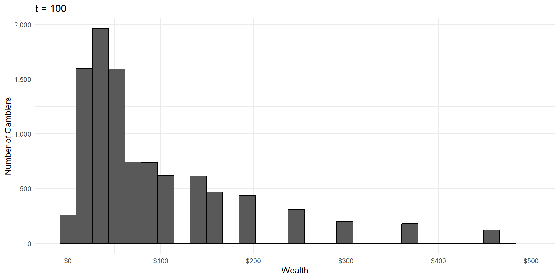
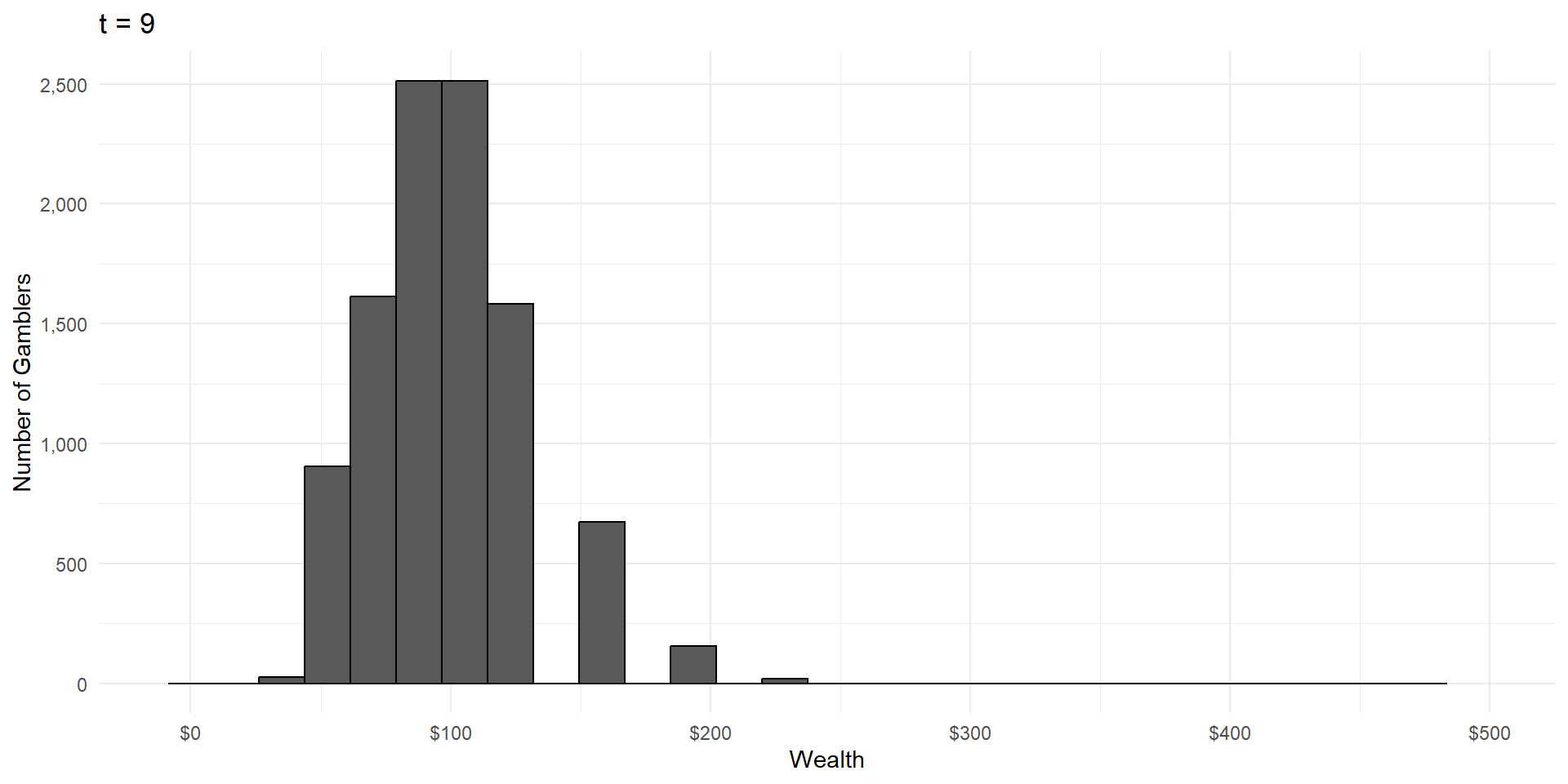
Violation 1: Multiplicative Processes
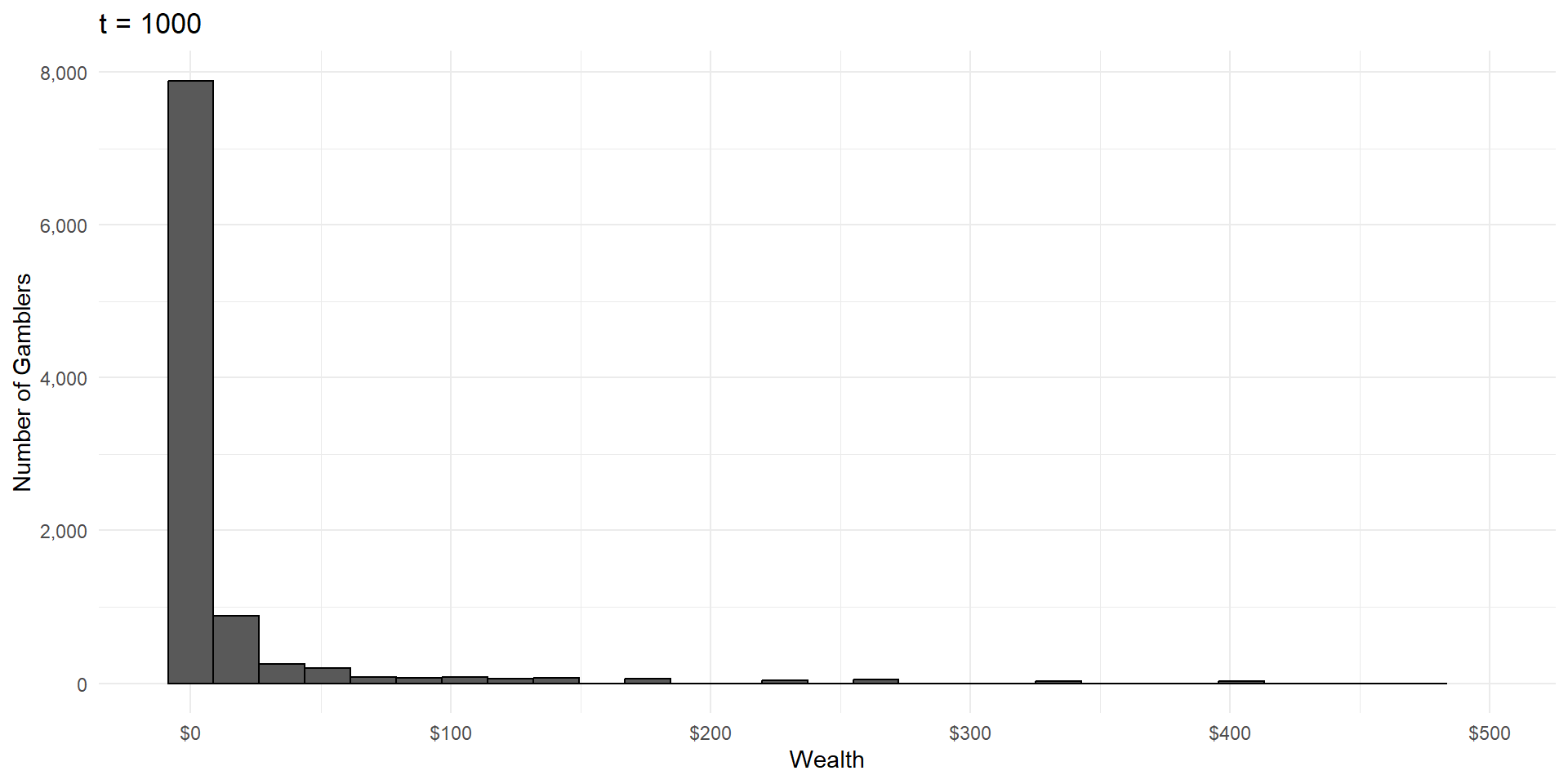
Violation 1: Multiplicative Processes
This is called a lognormal distribution, because here’s what it looks like on a logarithmic scale:
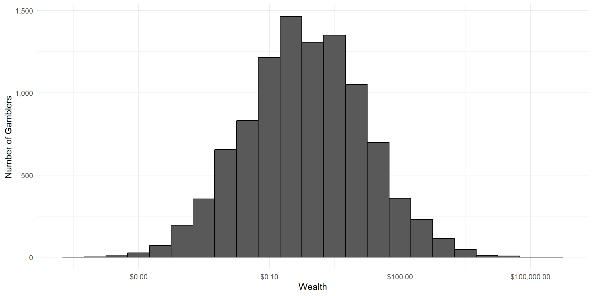
Lognormal Distributions
Lognormal Distributions
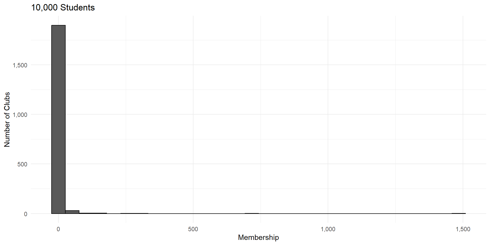
Violation 2: Interdependence
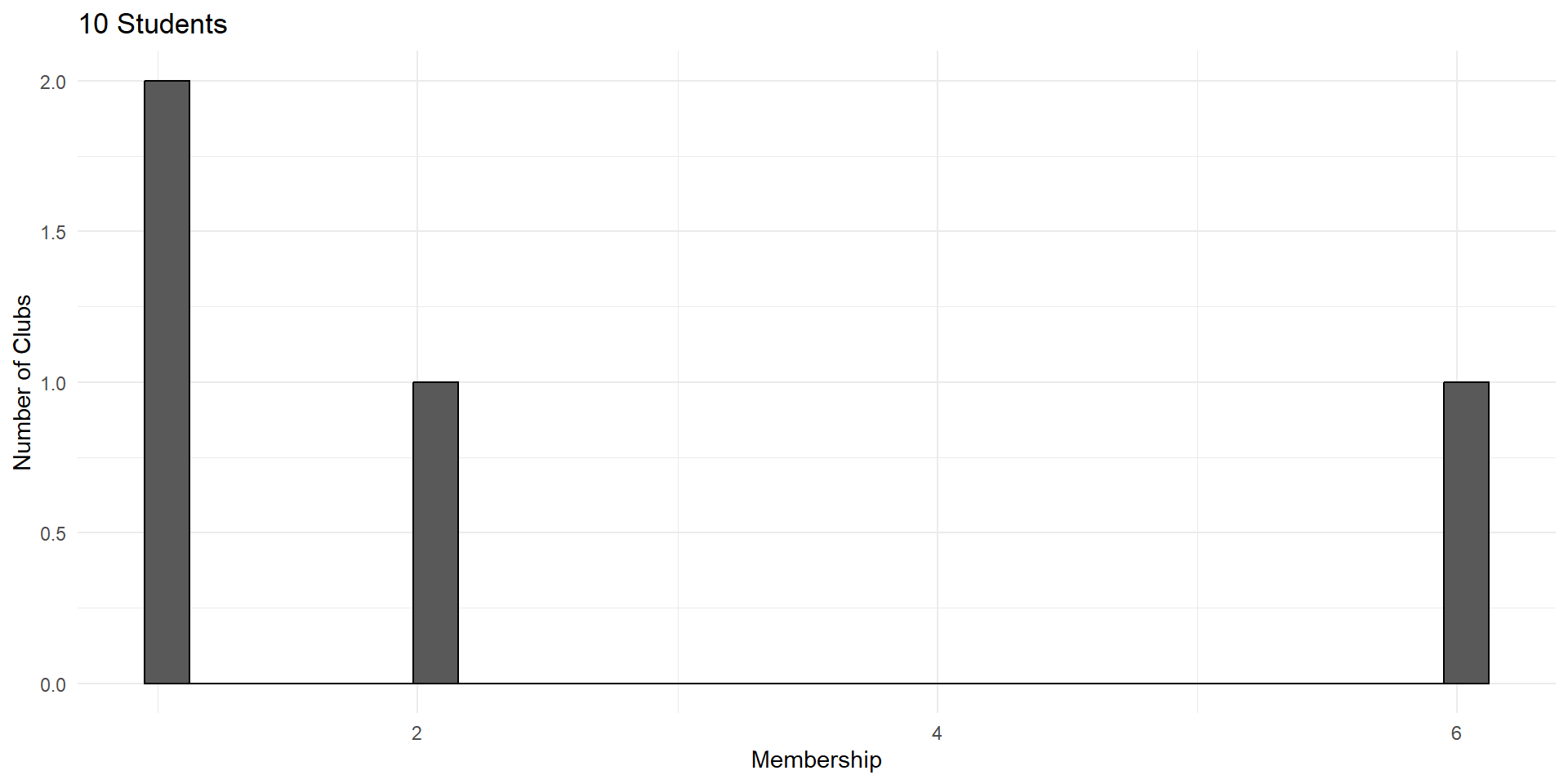
Violation 2: Interdependence
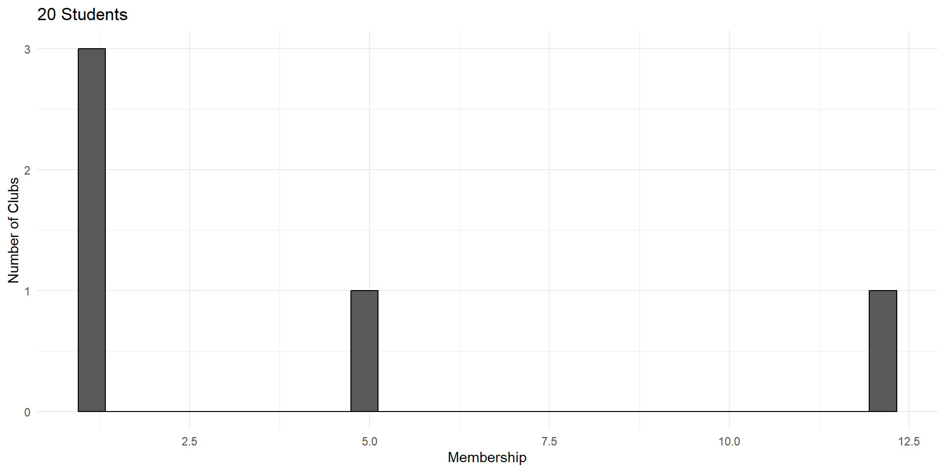
Violation 2: Interdependence
Violation 2: Interdependence
Violation 2: Interdependence
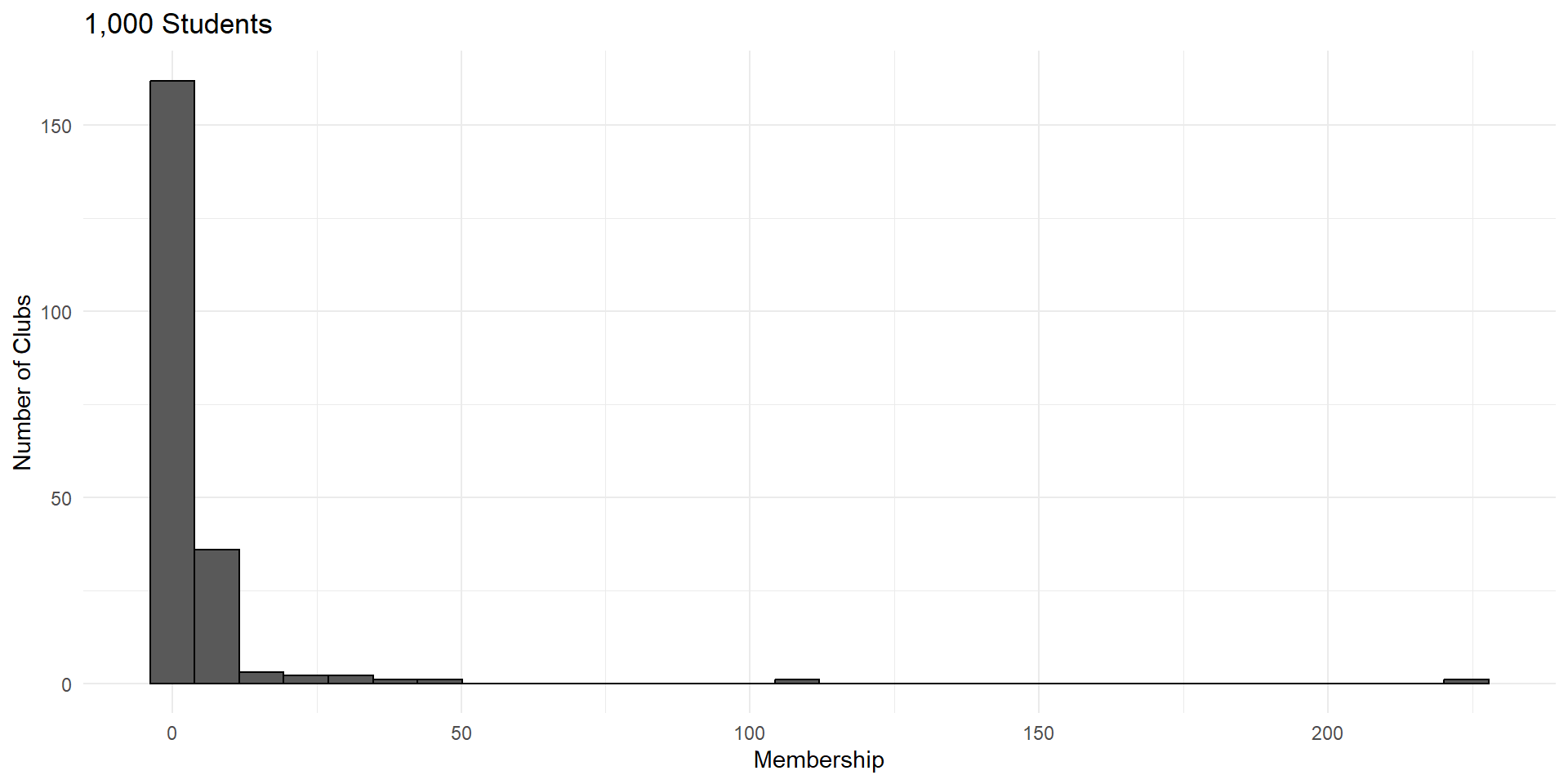
Violation 2: Interdependence
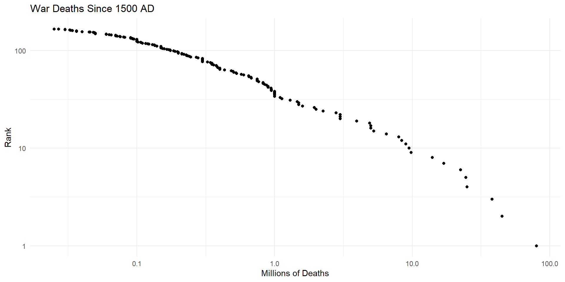
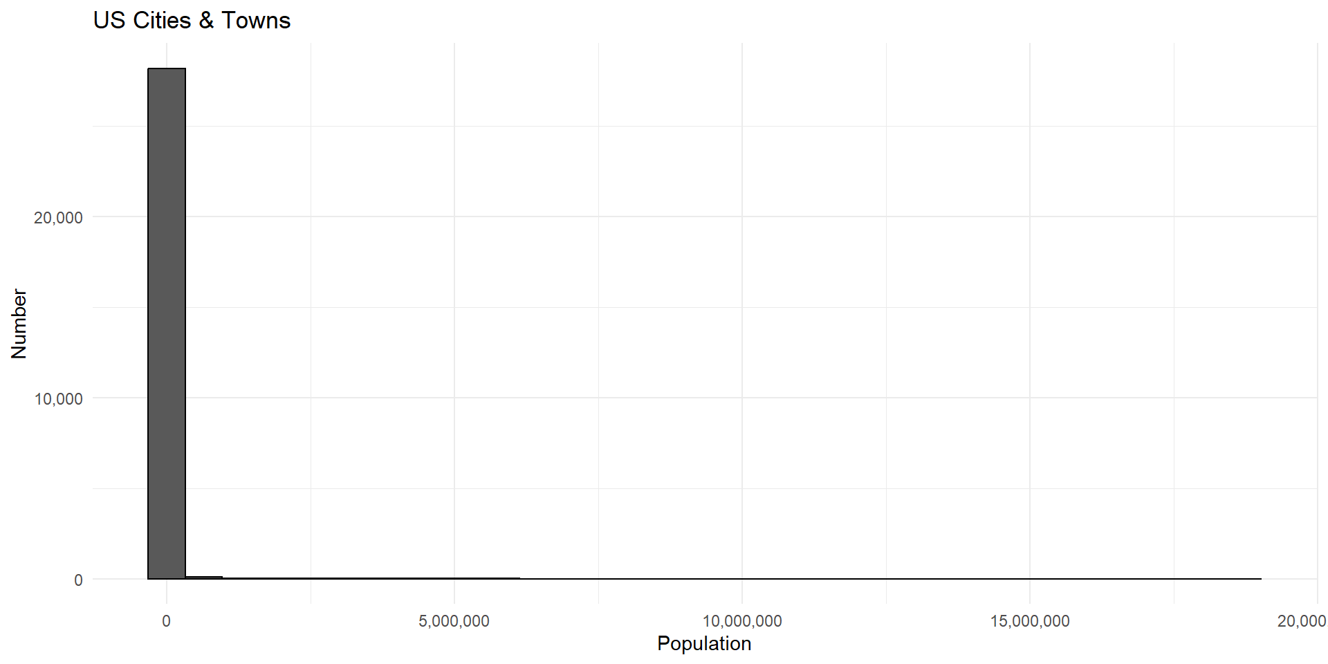
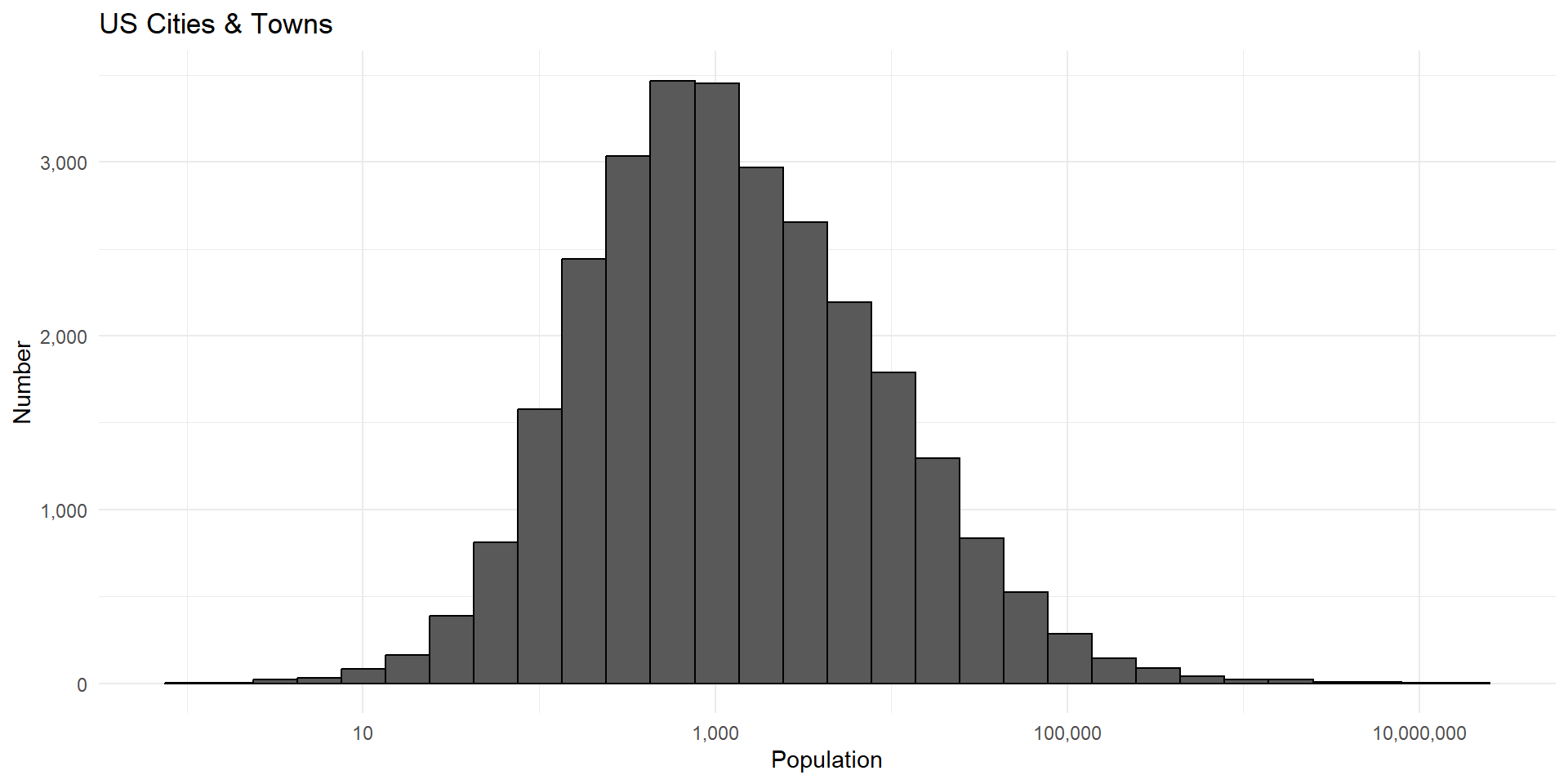
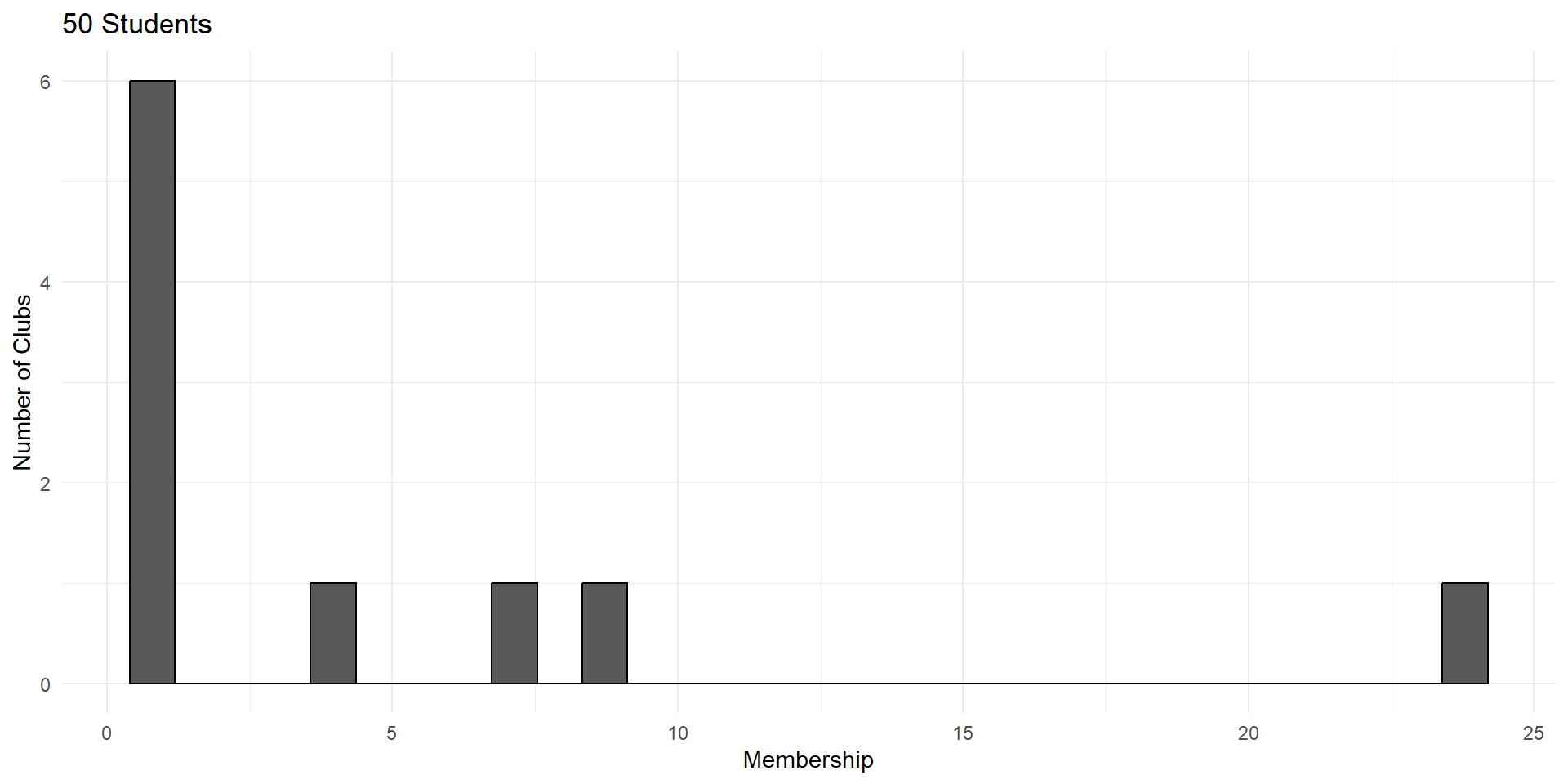
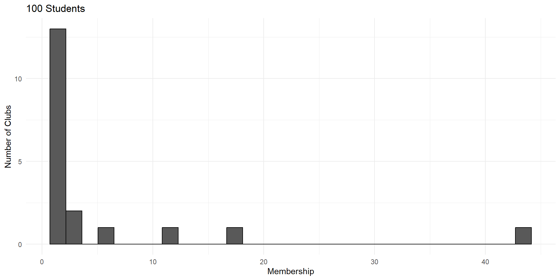
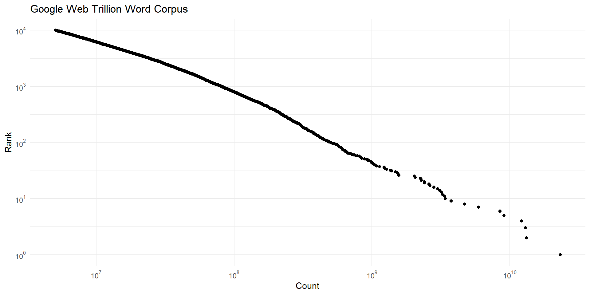
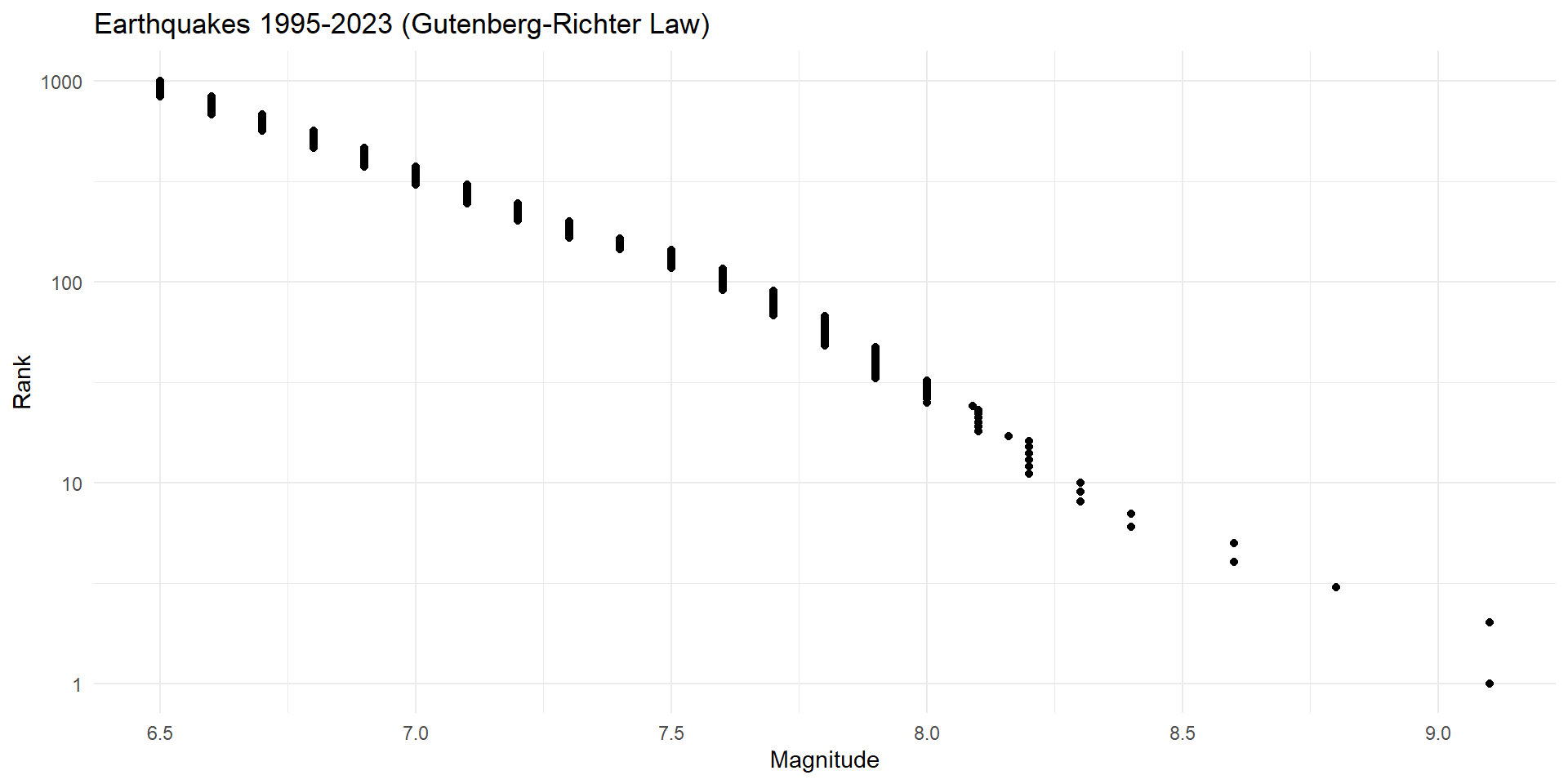
Power Laws
Distributions generated by this type of process are called power laws. They have a very distinct shape.
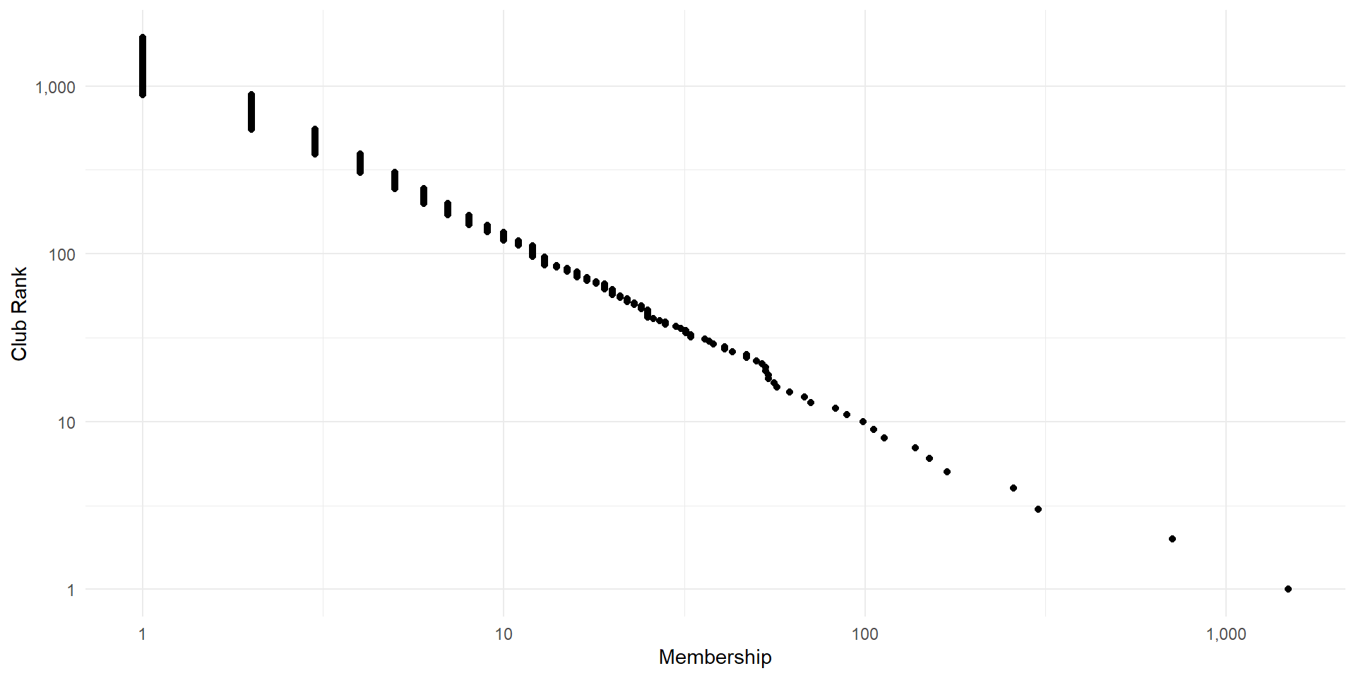
Power Laws
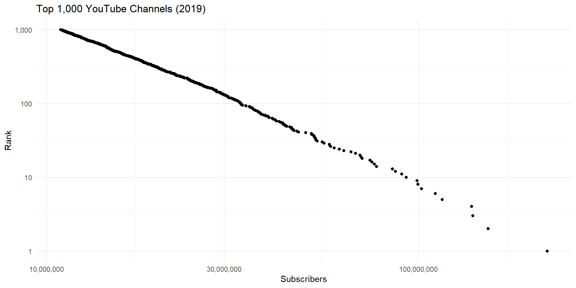
Power Laws
Power Laws
Power Laws