  midterm final overall gradeA
1   79.25 47.00    69.2      0
2   96.25 87.75    94.3      1
3   58.25 37.75    62.0      0
4   54.50 62.00    72.4      0
5   83.00 39.75    72.4      0
6 41.75 49.50 59.5 0Calculus Essentials
Derivatives & Optimization
The Linear Model
For this demonstration, download the grades.csv dataset.
The Linear Model
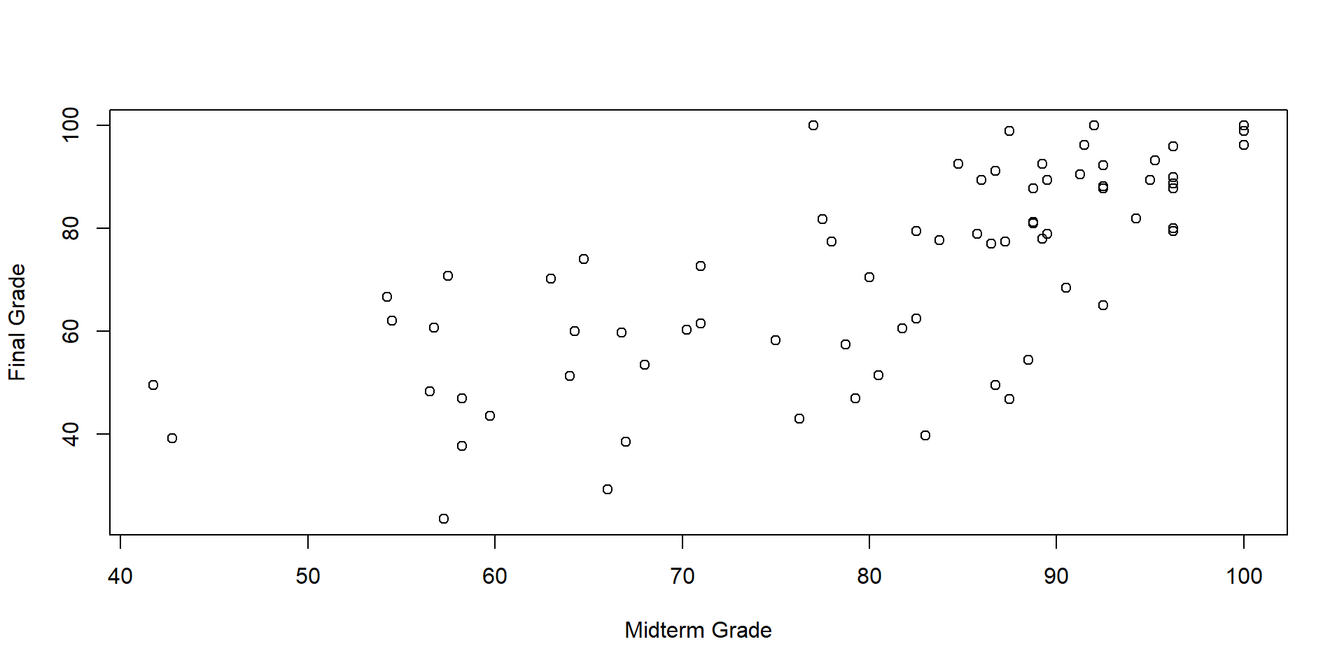
The Linear Model

The Linear Model
\[ y_i = \alpha + \beta x_i + \varepsilon_i \]
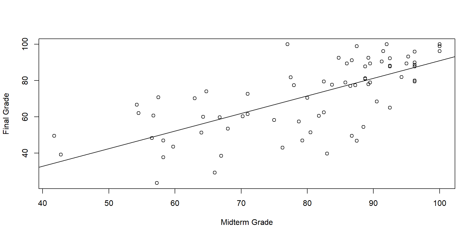
The Linear Model
Partitioning the outcome into two parts—the part we can explain, and the part we’re ignoring:
\[ \underbrace{y_i}_\text{outcome} = \underbrace{\alpha + \beta x_i}_\text{explained} + \underbrace{\varepsilon_i}_\text{unexplained} \]
The Linear Model
Partitioning the outcome into two parts—the part we can explain, and the part we’re ignoring:
\[ \underbrace{y_i}_\text{outcome} = \overbrace{\alpha}^\text{intercept parameter} + \beta x_i + \varepsilon_i \]
The Linear Model
Partitioning the outcome into two parts—the part we can explain, and the part we’re ignoring:
\[ \underbrace{y_i}_\text{outcome} = \overbrace{\alpha}^\text{intercept parameter} + \underbrace{\beta}_\text{slope parameter} x_i + \varepsilon_i \]
The Linear Model
Partitioning the outcome into two parts—the part we can explain, and the part we’re ignoring:
\[ \underbrace{y_i}_\text{outcome} = \overbrace{\alpha}^\text{intercept parameter} + \underbrace{\beta}_\text{slope parameter} \overbrace{x_i}^\text{explanatory variable} + \varepsilon_i \]
The Linear Model
Partitioning the outcome into two parts—the part we can explain, and the part we’re ignoring:
\[ \underbrace{y_i}_\text{outcome} = \overbrace{\alpha}^\text{intercept parameter} + \underbrace{\beta}_\text{slope parameter} \overbrace{x_i}^\text{explanatory variable} + \underbrace{\varepsilon_i}_\text{prediction error} \]
But where do the \(\alpha\) and \(\beta\) values come from? How do we estimate the “line of best fit”?
An Optimization Problem
We want to find values for \(\alpha\) and \(\beta\) that minimize the sum of squared error.
An Optimization Problem
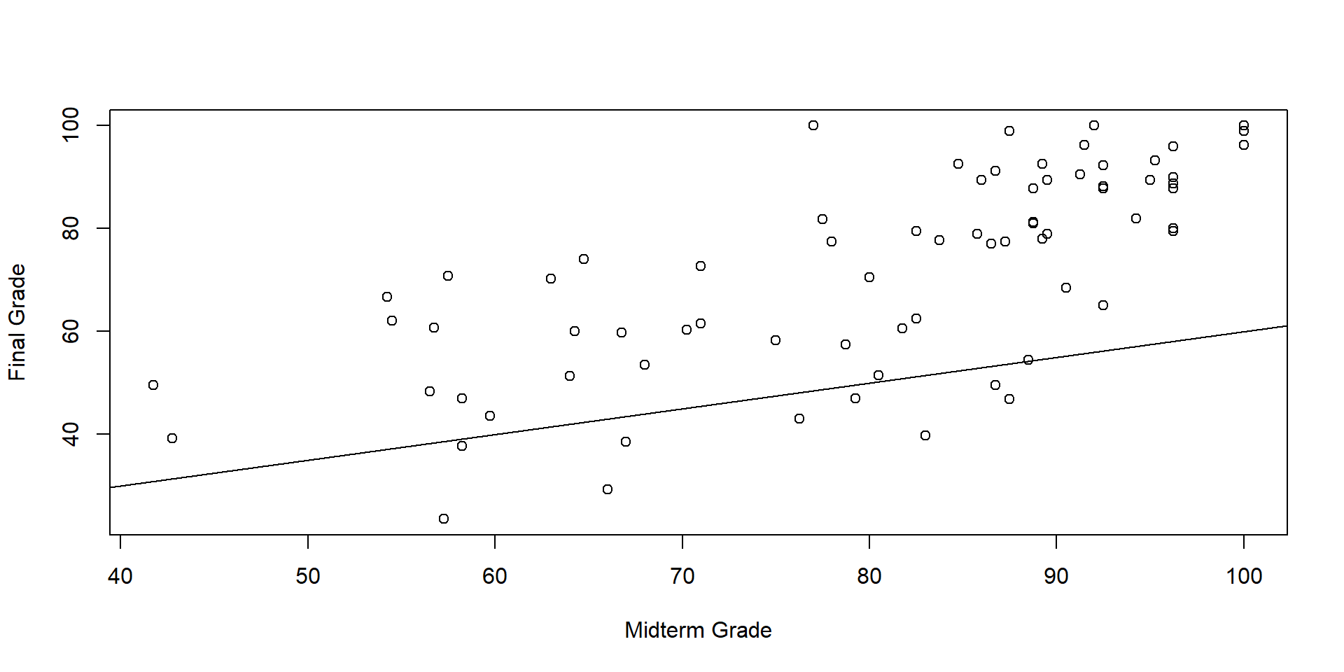
An Optimization Problem
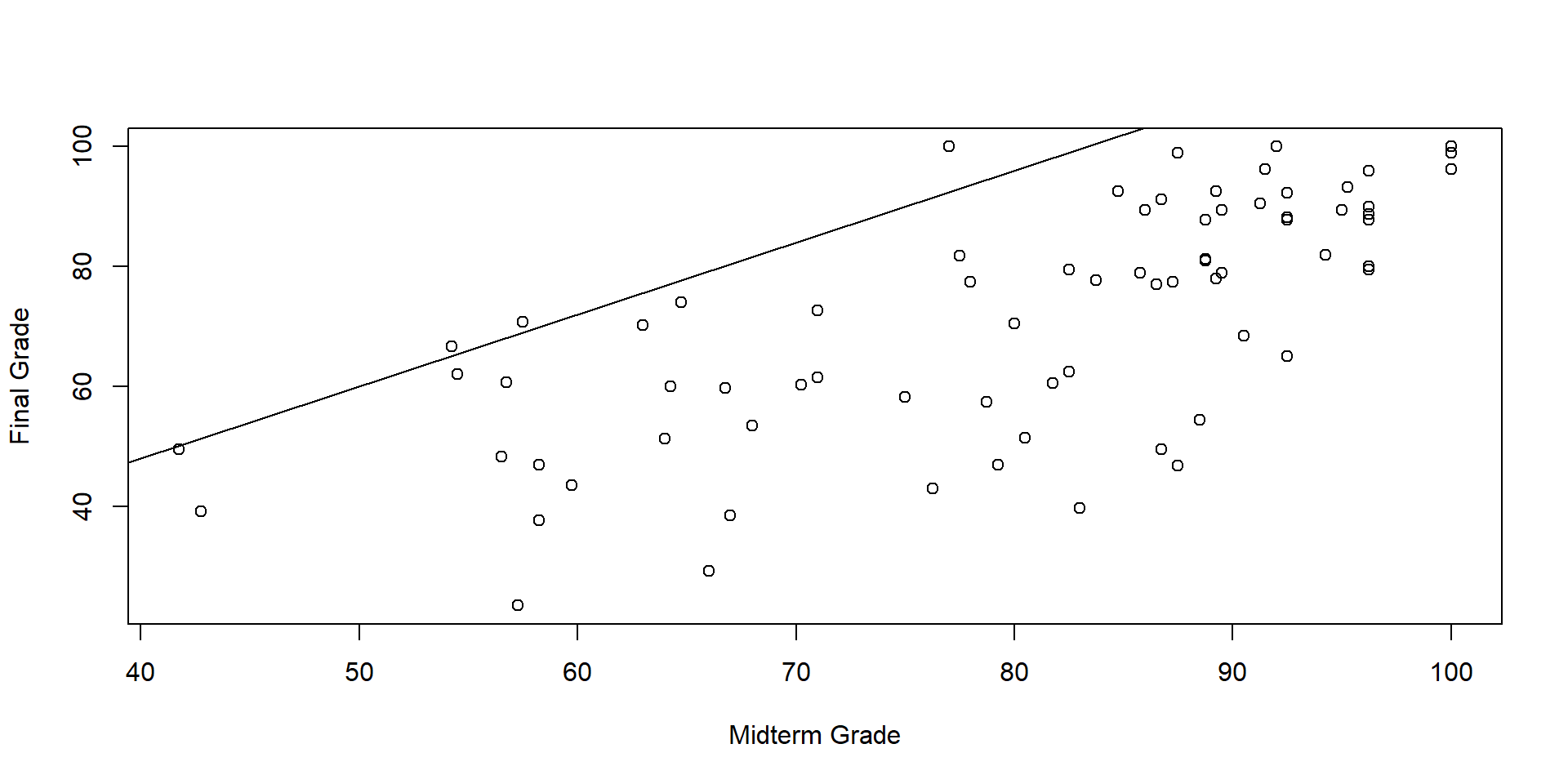
An Optimization Problem
We could keep hunting blindly for values \(\alpha\) and \(\beta\) that minimize the sum of squared errors, or we could take a more systematic approach…
\[ \text{SSE} = \sum_{i=1}^n(y_i - \alpha - \beta x_i)^2 \]
An Optimization Problem
\(\text{SSE} = \sum_{i=1}^n(y_i - \alpha - \beta x_i)^2\)
Imagine dropping a ball on this surface. The ball will roll until it reaches a perfectly flat point: the function’s minimum.
Review: Slopes
What is the slope of this function? \(f(x) = 3x + 2\)
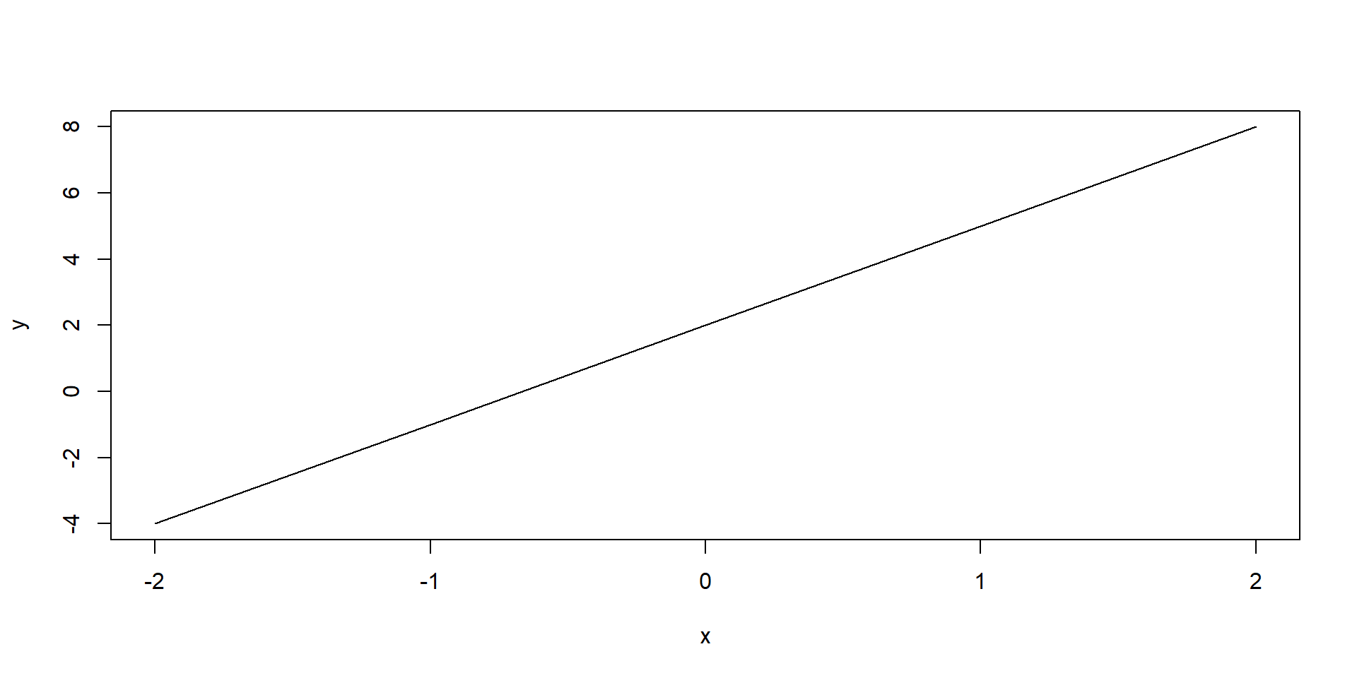
The slope of a linear function (a straight line) is measured by how much \(y\) increases when you increase \(x\) by \(1\). In this case, \(3\).
Review: Slopes
Find the slope of each function:
\(y = 2x + 4\)
\(f(x) = \frac{1}{2}x - 2\)
life expectancy (years) = 18.09359 + 5.737335 \(\times\) log(GDP per capita)
Slope of a line \(= \frac{rise}{run} = \frac{\Delta Y}{\Delta X} = \frac{f(x+h) - f(x)}{h}\)
Nonlinear Functions
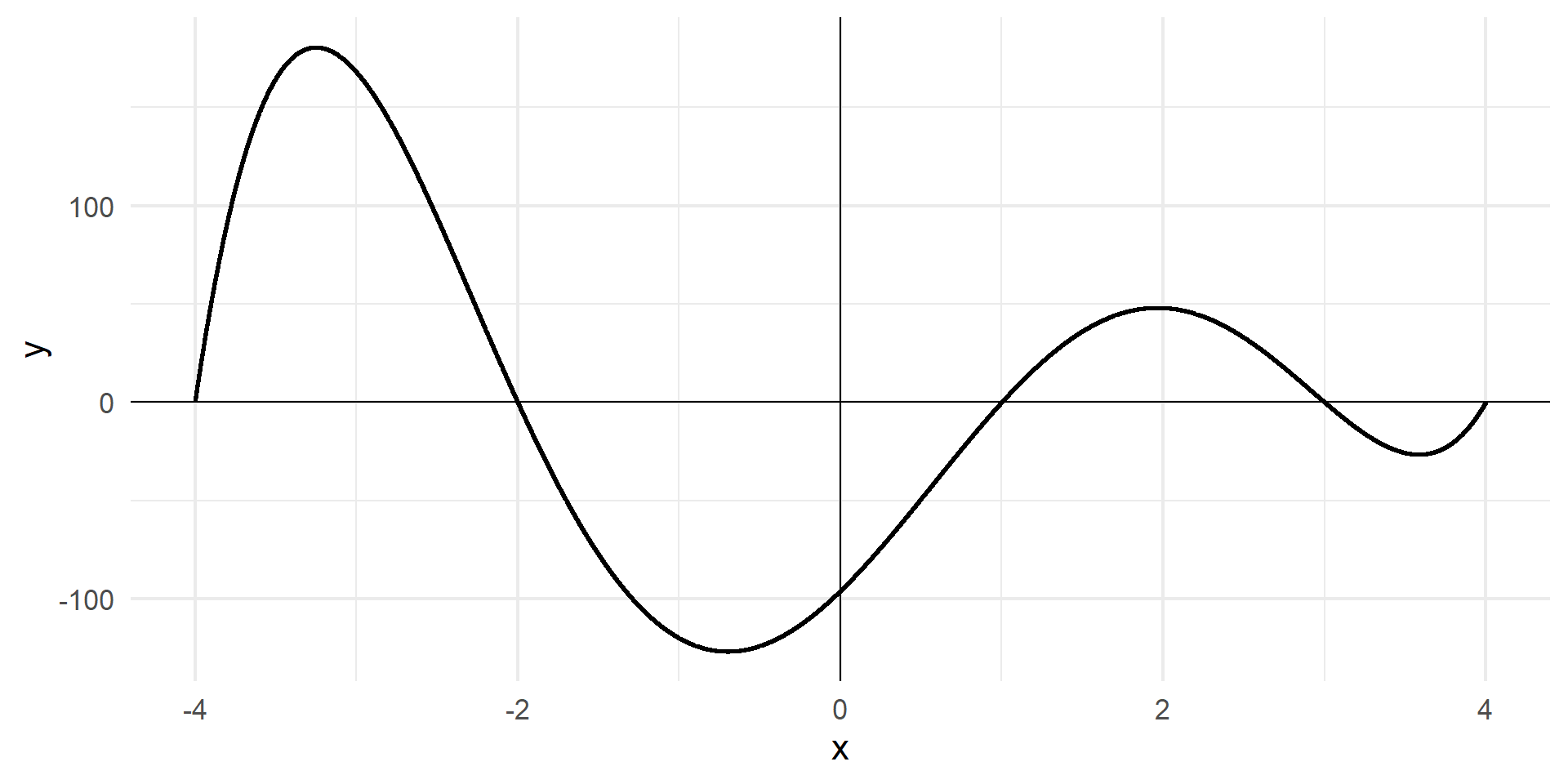
Nonlinear functions are confusing and scary…
Newton & Leibniz


The Key Insight
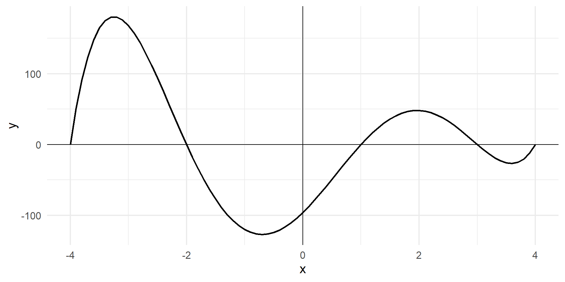
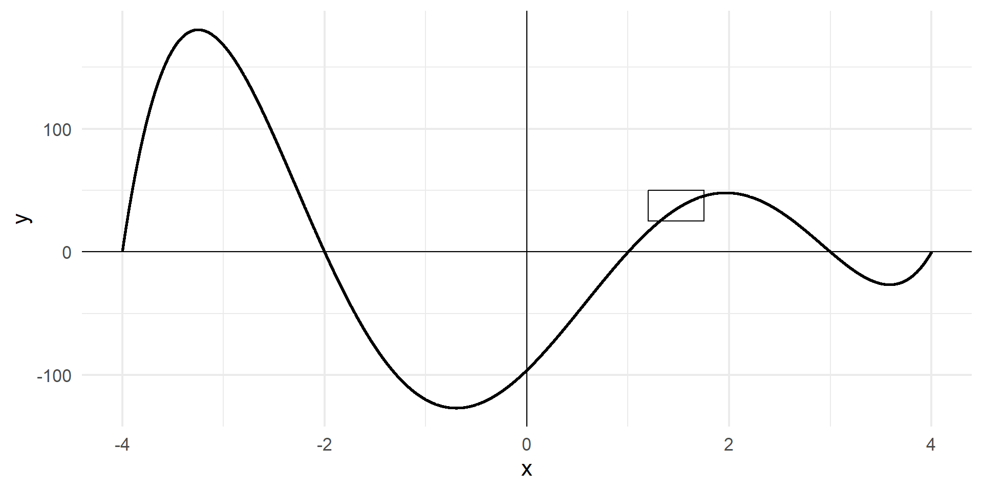
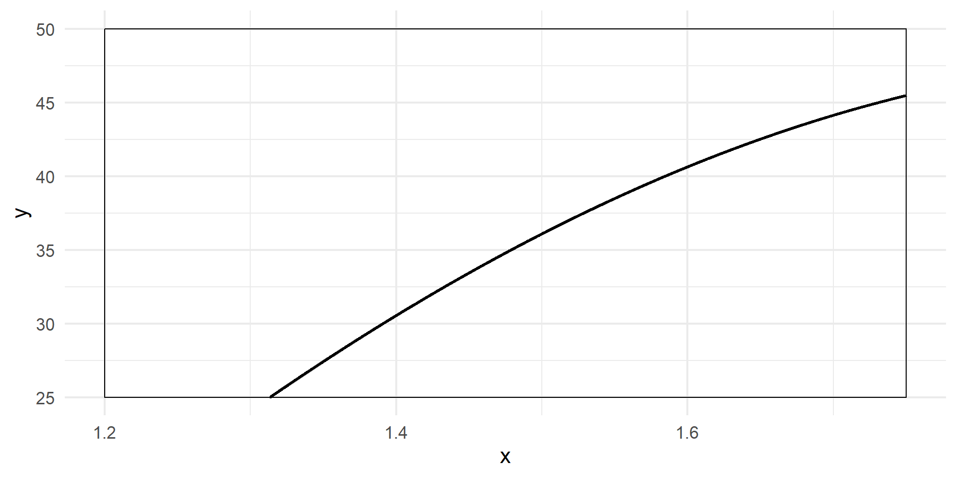
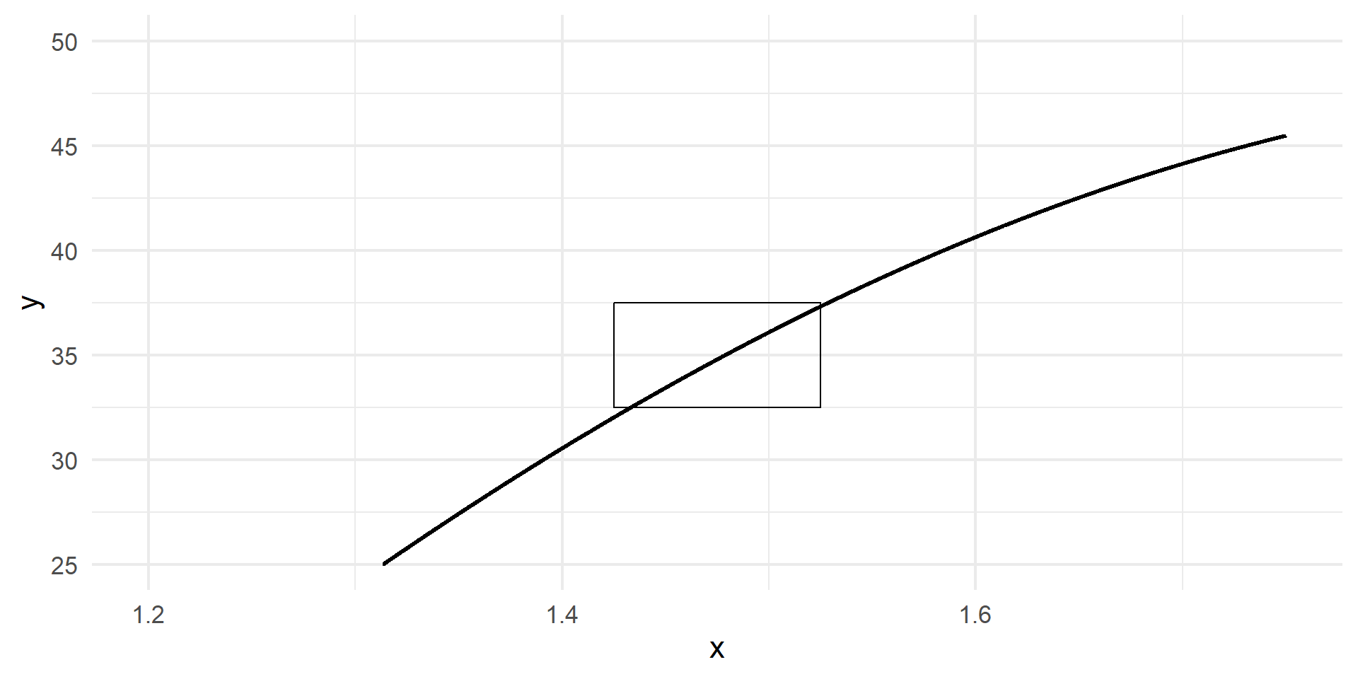
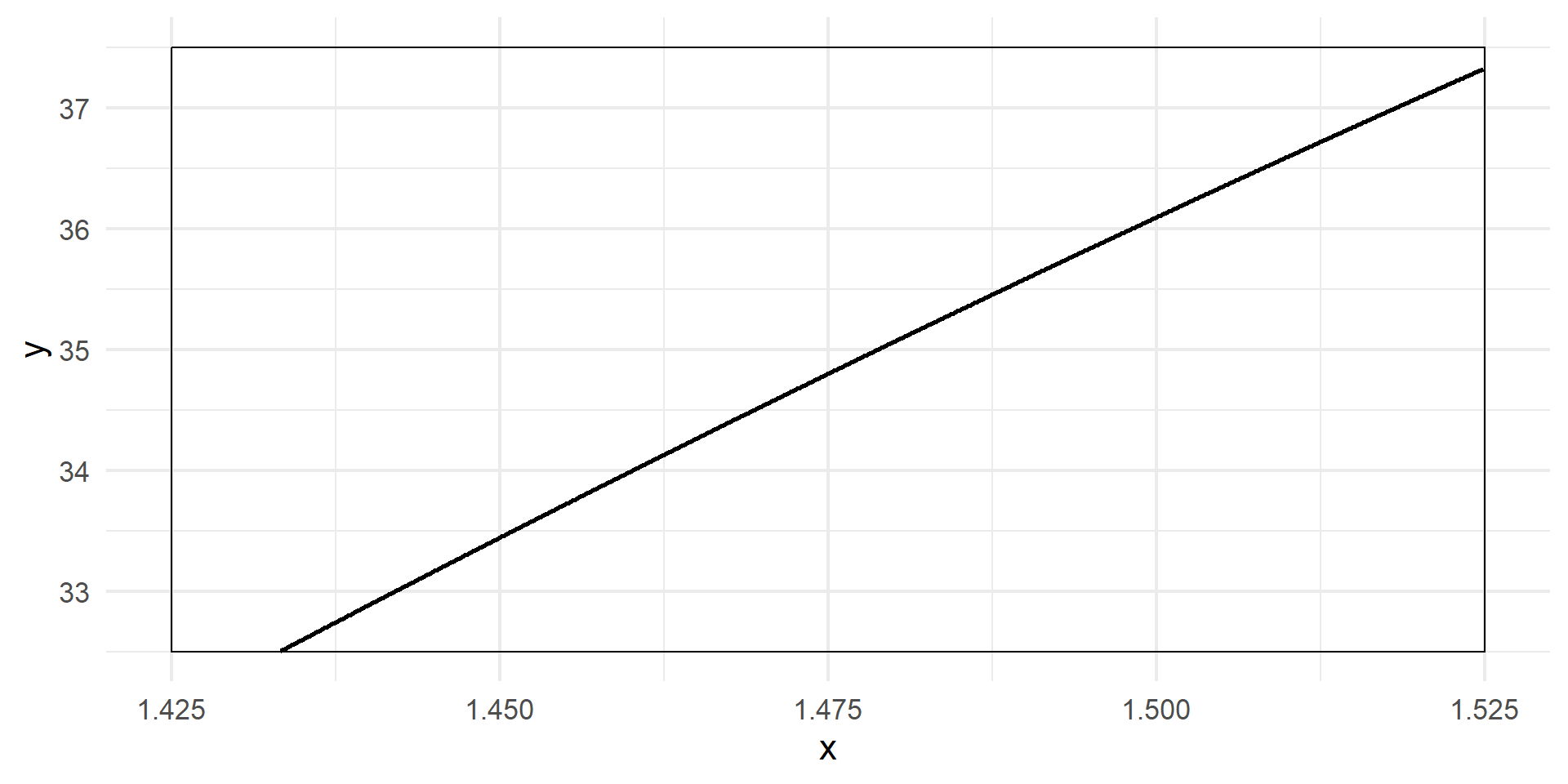
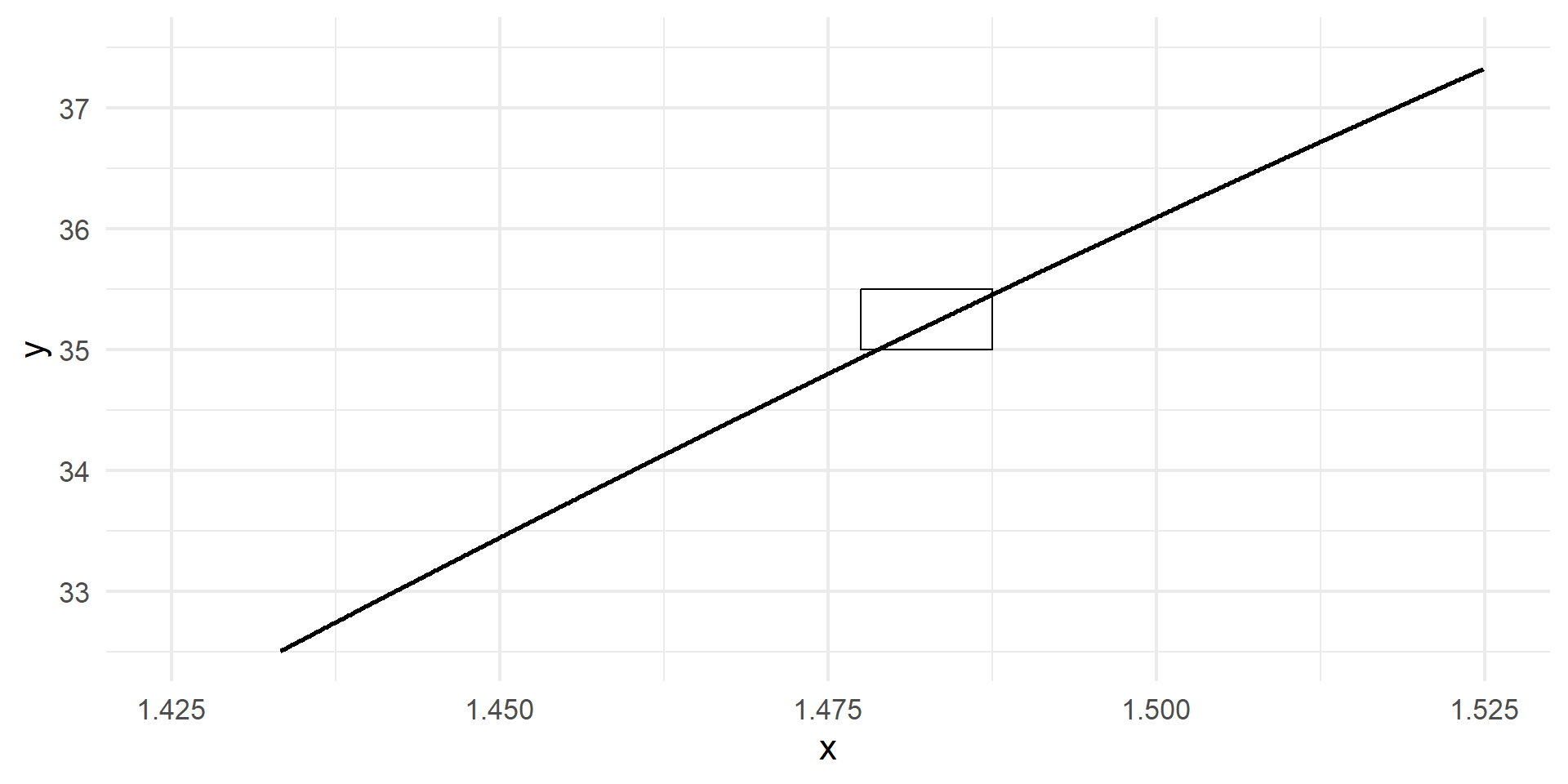
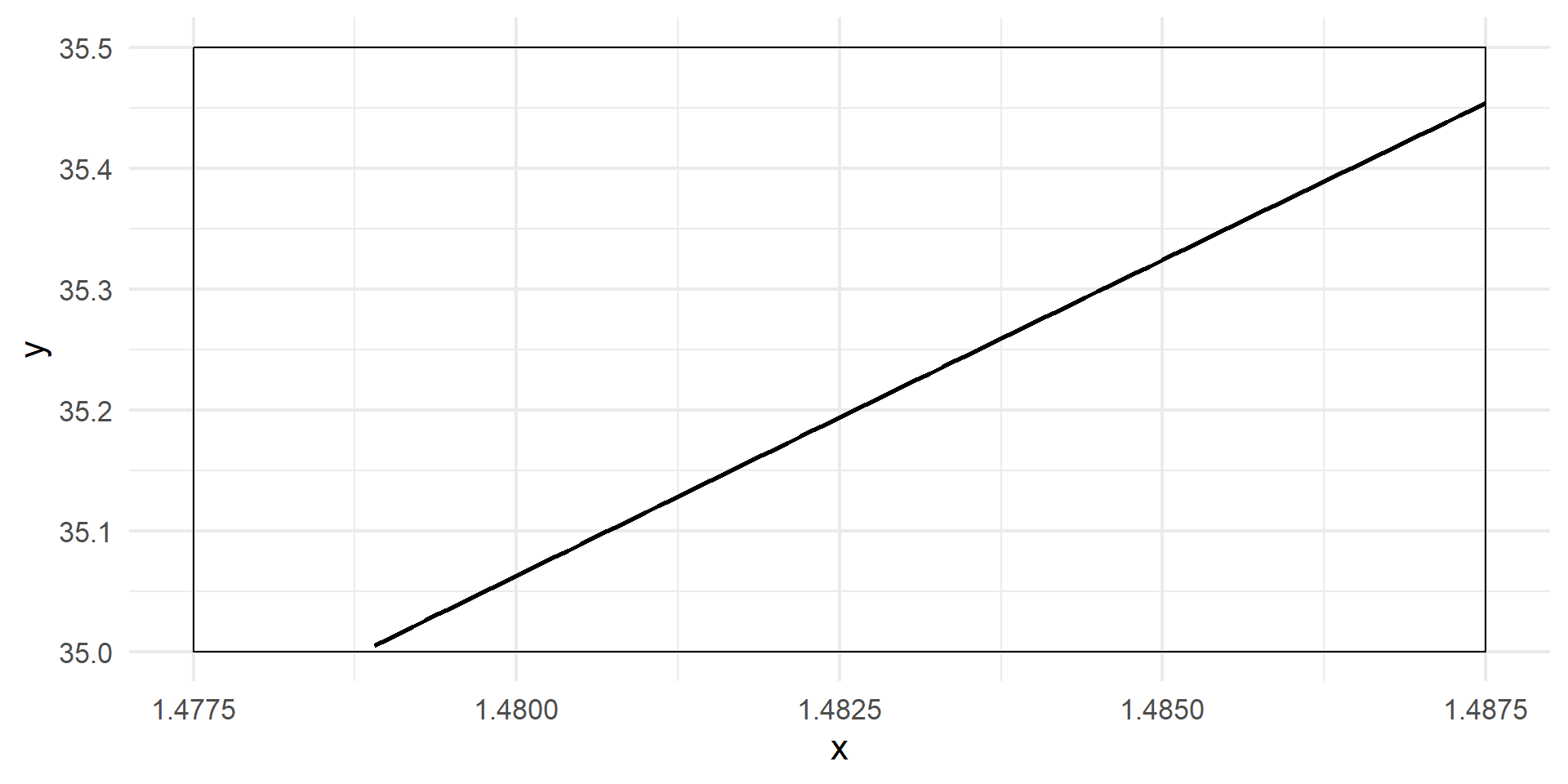
Any curve becomes a straight line if you “zoom in” far enough.
The Key Insight
Any curve becomes a straight line if you “zoom in” far enough.
The Key Insight
Any curve becomes a straight line if you “zoom in” far enough.
The Key Insight
Any curve becomes a straight line if you “zoom in” far enough.
The Key Insight
Any curve becomes a straight line if you “zoom in” far enough.
The Key Insight
Any curve becomes a straight line if you “zoom in” far enough.
The Key Insight
Any curve becomes a straight line if you “zoom in” far enough.
The Key Insight

Putting all that into math…
\[ f'(x) = \lim_{h \to 0}\frac{f(x+h)-f(x)}{h} \]
Putting all that into math…
\[ f'(x) = \underbrace{\lim_{h \to 0}}_\text{shrink h really small}\frac{\overbrace{f(x+h)-f(x)}^\text{the change in y}}{\underbrace{h}_\text{the change in x}} \]
This is called the derivative of a function. Using the derivative, you can find the slope at any point.
Derivative Example
Let \(f(x) = 2x + 3\). What is \(f'(x)\)?
\[ f'(x) = \lim_{h \to 0}\frac{f(x+h)-f(x)}{h} \]
\[ = \lim_{h \to 0}\frac{2(x+h)+3-(2x+3)}{h} \]
\[ = \lim_{h \to 0}\frac{2x+2h+3-(2x+3)}{h} \]
Derivative Example
Let \(f(x) = 2x + 3\). What is \(f'(x)\)?
\[ = \lim_{h \to 0}\frac{2x+2h+3-(2x+3)}{h} \]
\[ = \lim_{h \to 0}\frac{2h}{h} \]
\[ = 2 \]
Now A Nonlinear Example
Let \(f(x) = 3x^2 + 2x + 3\). What is \(f'(x)\)?
\[ = \lim_{h \to 0}\frac{3(x+h)^2 + 2(x+h) + 3 - (3x^2 + 2x + 3)}{h} \]
\[ = \lim_{h \to 0}\frac{3x^2 + 3h^2 + 6xh + 2x+ 2h + 3 - (3x^2 + 2x + 3)}{h} \]
\[ = \lim_{h \to 0}\frac{3h^2 + 6xh + 2h}{h} \]
Now A Nonlinear Example
Let \(f(x) = 3x^2 + 2x + 3\). What is \(f'(x)\)?
\[ = \lim_{h \to 0}\frac{3h^2 + 6xh + 2h}{h} \]
\[ = \lim_{h \to 0}3h + 6x + 2 \]
\[ = 6x + 2 \]
Solution
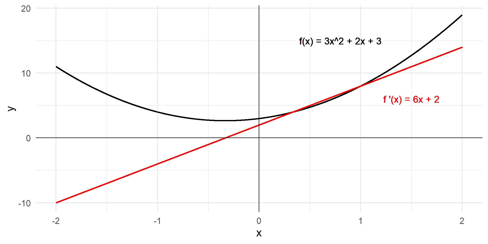
The function \(f'(x)\), outputs the slope of \(f(x)\) at every point.
Derivative Shortcuts
Good news! You don’t have to go through that process every time. Mathematicians have done it for you, and have discovered a whole bunch of useful shortcuts.
Shortcut 1: The Power Rule
If \(f(x) = ax^k\), then \(f'(x) = kax^{k-1}\)
Example: If \(f(x) = 5x^4\), then \(f'(x) = 20x^3\).
Practice Problem: Let \(f(x) = 2x^3\). What is \(f'(x)\)?
\[f'(x) = 6x^2\]
Shortcut 2: The Sum Rule
The derivative of a sum is equal to the sum of derivatives.
If \(f(x) = g(x) + h(x)\), then \(f'(x) = g'(x) + h'(x)\)
Example: If \(f(x) = x^3 + x^2\), then \(f'(x) = 3x^2 + 2x\)
Practice Problem: If \(f(x) = 2x^3 + x^2\), what is \(f'(x)\)?
\[f'(x) = 6x^2 + 2x\]
Shortcut 3: The Constant Rule
The derivative of a constant is zero.
If \(f(x) = c\), then \(f'(x) = 0\)
Example: If \(f(x) = 5\), then \(f'(x) = 0\).
Practice Problem: If \(f(x) = 4x^2 + 3x + 5\), what is \(f'(x)\)?
\[ f'(x) = 8x + 3 \]
Shortcut 4: The Product Rule
The derivative of a product is a bit trickier…
If \(f(x) = g(x) \cdot h(x)\), then \(f'(x) = g'(x) \cdot h(x) + g(x) \cdot h'(x)\)
Example: If \(f(x) = (2x)(x + 2)\), then \(f'(x) = 2x + 2(x+2) = 4x + 4\)
Practice Problem: \(f(x) = (3x^2 + 6x)(x+2)\), what is \(f'(x)\)?
\[f'(x) = (3x^2 + 6x)(1) + (6x + 6)(x+2)\]
\[f'(x) = 3x^2 + 6x + 6x^2 + 6x + 12x + 12\]
\[f'(x) = 9x^2 + 24x + 12\]
Shortcut 5: The Chain Rule
If \(f(x) = g(h(x))\), then \(f'(x) = g'(x) \cdot h'(x)\)
“The derivative of the outside times the derivative of the inside.”
Example: If \(f(x) = (2x^2 - x + 1)^3\), then \(f'(x) = 3(2x^2 - x + 1)^2 (4x - 1)\)
Practice Problem: \(f(x) = \sqrt{x + 3} = (x+3)^{\frac{1}{2}}\), what is \(f'(x)\)?
\(f'(x) = \frac{1}{2}(x+3)^{-\frac{1}{2}}(1) = \frac{1}{2\sqrt{x+3}}\)
More Practice
- Let \(f(x) = 2x^3 + 4x + 79\). What is \(f'(x)\)?
- Let \(f(x) = 3(x^2 + x + 42)\). What is \(f'(x)\)?
- Let \(f(x) = (x^2 + 1)(x+3)\). What is \(f'(x)\)?
Now We Can Do Optimization!
Let \(f(x) = 2x^2 + 8x - 32\). At what value of \(x\) is the function minimized?
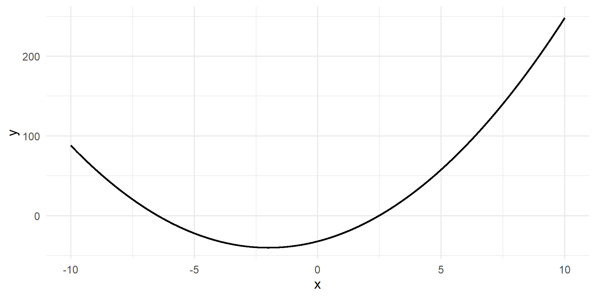
Key Insight: Function is minimized when the slope “switches” from decreasing to increasing. Exactly at the point where the slope equals zero.
Optimization in Three Steps
1. Take the derivative of the function.
2. Set it equal to zero.
3. Solve for \(x\).
Optimization in Three Steps
1. Take the derivative of the function.
\[ f(x) = 2x^2 + 8x - 32 \]
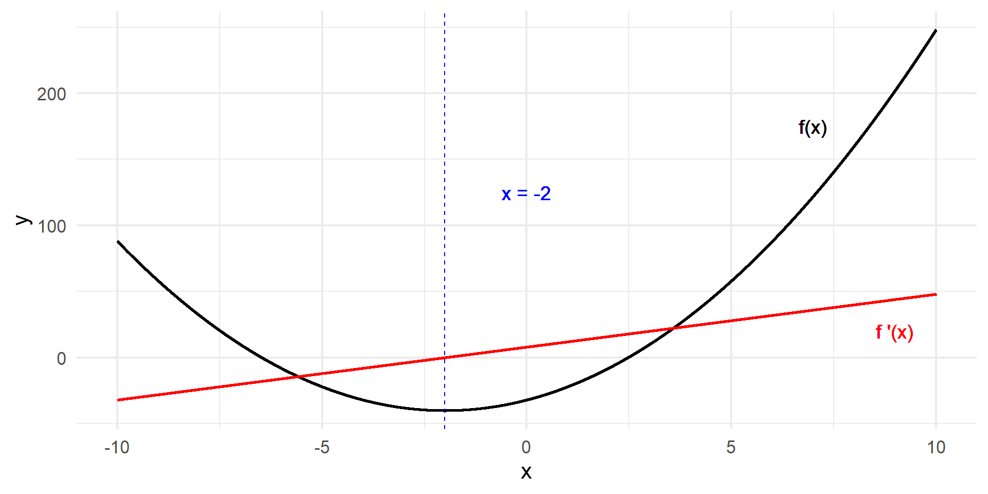
\[ f'(x) = 4x + 8 \]
2. Set it equal to zero
\[ 4x + 8 = 0 \]
3. Solve for \(x\).
\[ x = -2 \]
Optimization in Three Steps
Now You Try It!
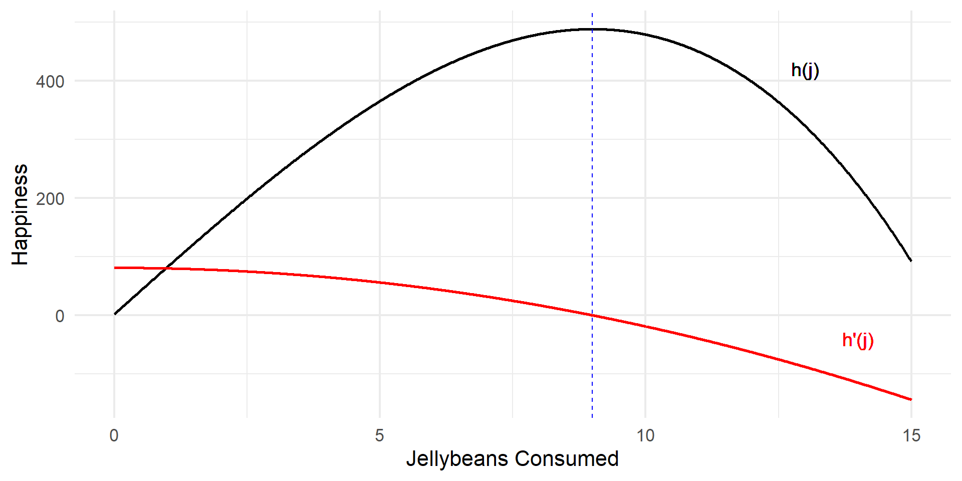
Suppose that happiness as a function of jellybeans consumed is \(h(j) = -\frac{1}{3}j^3 + 81j + 2\). How many jellybeans should you eat? (Assume you can only eat a positive number of jellybeans).
Now You Try It!
Suppose that happiness as a function of jellybeans consumed is \(h(j) = -\frac{1}{3}j^3 + 81j + 2\). How many jellybeans should you eat? (Assume you can only eat a positive number of jellybeans).
Wait.
How do you know if it’s a maximum or a minimum?
\(h(j) = \frac{1}{3}j^3 + 81j + 2\) and \(h'(j) = 81 - j^2\)

Wait.
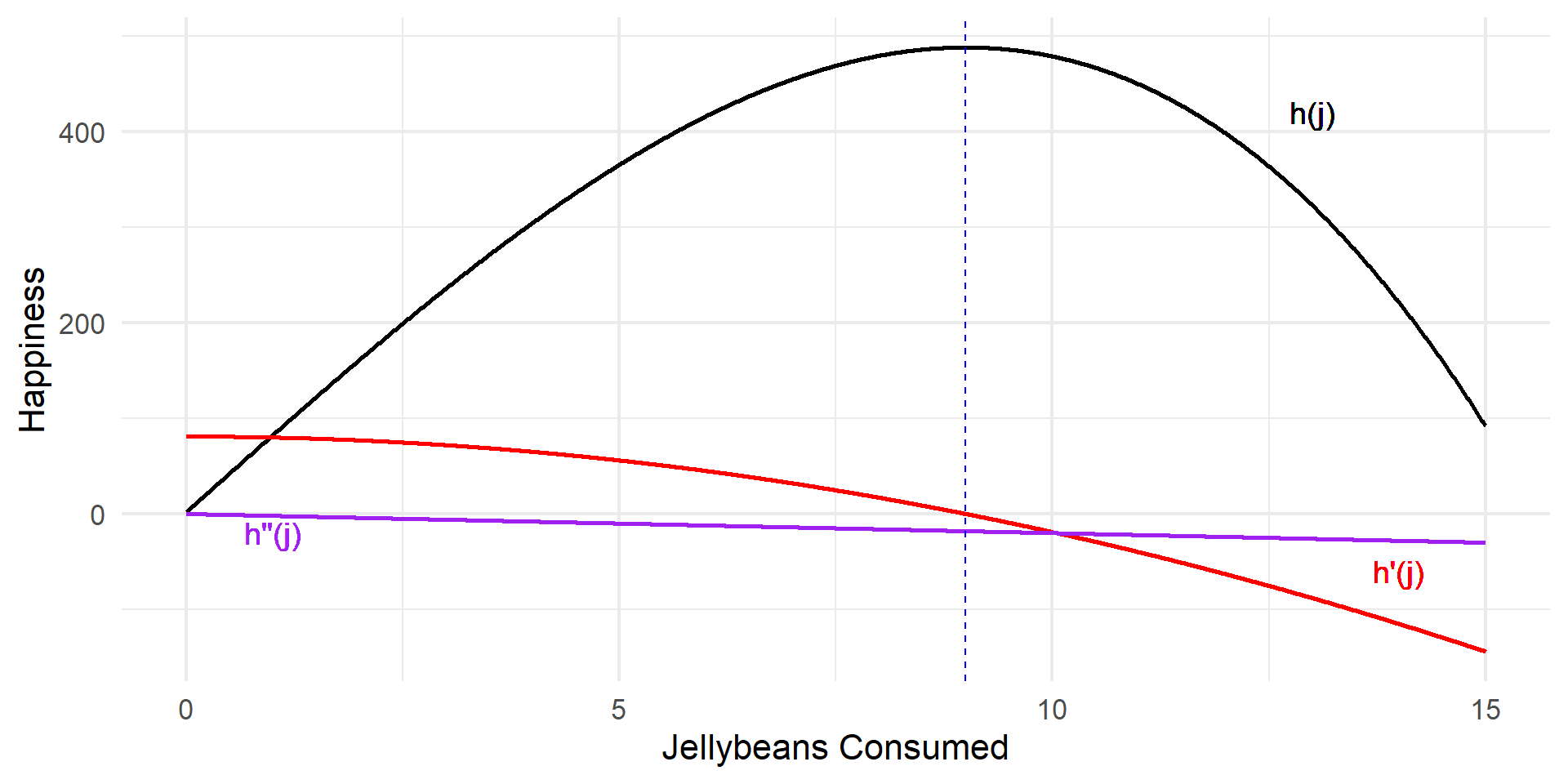
It’s a maximum when the slope is decreasing, and a minimum when then slope is increasing. How do you figure out if the slope is increasing or decreasing?
That’s right. You find the slope of the slope (the derivative of the derivative, aka the second derivative).
The Second Derivative Test
\(h(j) = \frac{1}{3}j^3 + 81j + 2\) and \(h'(j) = 81 - j^2\)
What is \(h''(j)\)? Is it positive or negative when you eat \(9\) jellybeans?
The Second Derivative Test
\(h(j) = \frac{1}{3}j^3 + 81j + 2\) and \(h'(j) = 81 - j^2\)
What is \(h''(j)\)? Is it positive or negative when you eat \(9\) jellybeans? \[ h''(j) = -2j \]
The Second Derivative Test
Partial Derivatives
What if you have a multivariable function?
\[ f(x,y) = 2x^2y + xy - 4x + y -6 \]
Same procedure! To get the derivative of a function with respect to \(x\) or \(y\), treat the other variable as a constant.
\[ \frac{\partial f}{\partial x} = 4yx + y - 4 \]
\[ \frac{\partial f}{\partial y} = 2x^2 + x + 1 \]
Now You Try!
Suppose happiness as a function of jellybeans and Dr. Peppers consumed is
\[h(j,d) = 8j -\frac{1}{2}j^2 + 2d - 3d^2 + jd + 100\]
How many jellybeans should you eat? How many Dr. Peppers should you drink?
Now You Try!
\[ h(j,d) = 8j -\frac{1}{2}j^2 + 2d - 3d^2 + jd + 100 \]
\[ \frac{\partial h}{\partial j} = 8 - j + d = 0 \]
\[ \frac{\partial h}{\partial d} = 2 - 6d + j = 0 \]
\[ j = 8 + d \]
\[ j = 6d - 2 \]
\[ d^* = 2 \]
\[ j^* = 10 \]
\[h(j,d) = 8j -\frac{1}{2}j^2 + 2d - 3d^2 + jd + 100\]
Next Week…
We finally have the tools we need to find the values of \(\alpha\) and \(\beta\) that minimize this function:
\(\text{SSE} = \sum_{i=1}^n(y_i - \alpha - \beta x_i)^2\)