Week 11: Data Tidying

This week we discuss the core principles of tidy data, and why you want to ensure that your data is tidy prior to conducting your statistical analyses. By the end of this week, you will be able to:

• Pivot datasets to change the unit of analysis

• Assess whether a dataset meets the three criteria necessary to be considered “tidy”

• Complete the steps necessary to convert a raw, “messy” dataset into a form amenable to statistical analysis

Reading

• R4DS Chapters 5-6

Problem Set

This dataset that I downloaded from the World Bank has extensive data on each country’s GDP per capita going back to the 1960s. But it’s hopelessly untidy. In this problem set, we’ll tidy it so that the unit of analysis is the country-year, then perform a few analyses.

1. Load the data into R. Note that the data itself doesn’t start until row 5, so you’ll need to account for that (hint: check out the skip argument in read.csv()).
2. Pivot the dataset so that each row is a country-year (e.g. Peru 1970), and there is a single column with the GDP per capita variable.
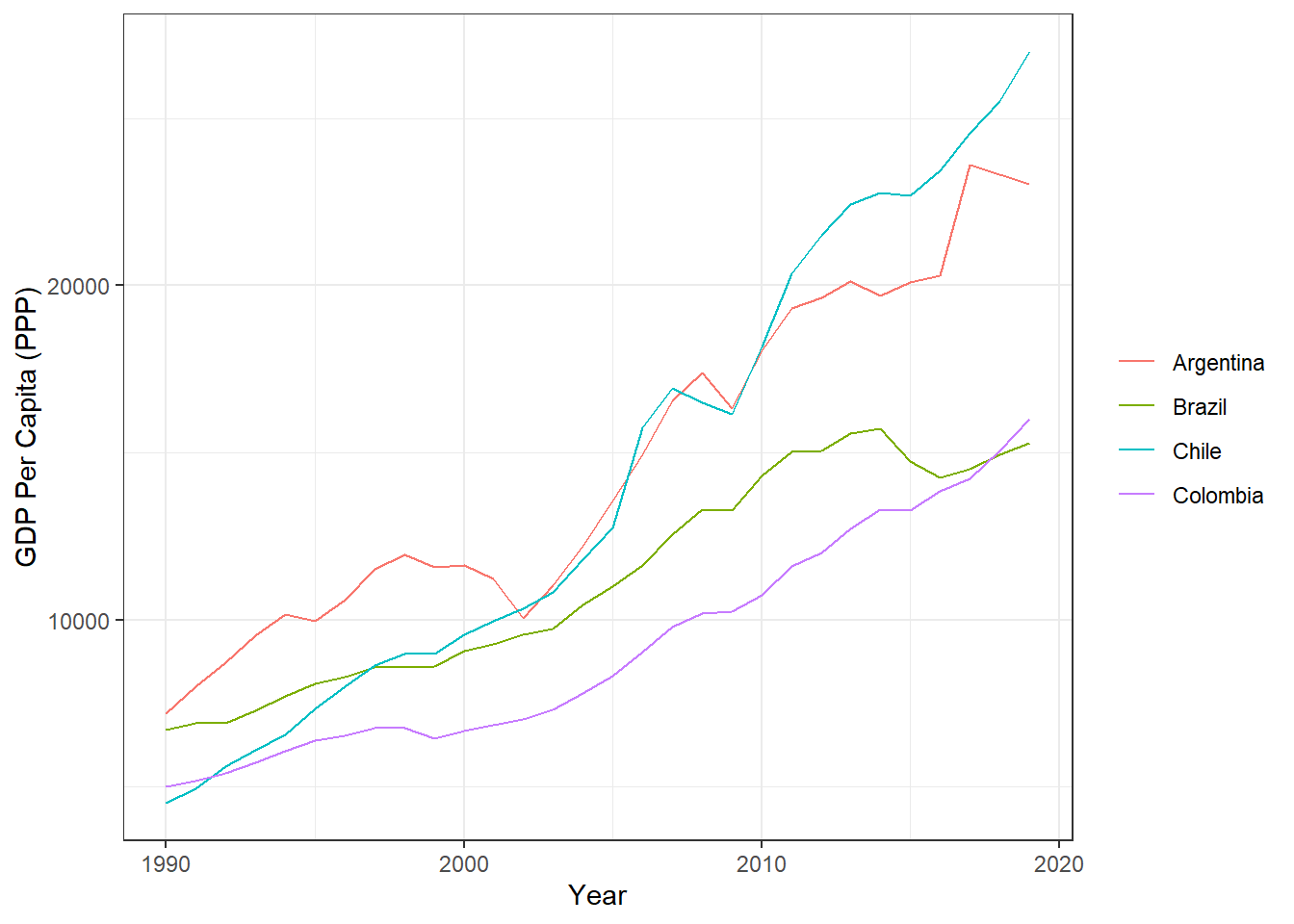
3. Make sure that the resulting year variable is formatted correctly as a numeric. (Hint: the str_remove_all() function may be helpful, depending on how you imported the dataset.)
4. Reproduce the following chart.

6. Bonus. Some economic growth theories suggest that poor countries should grow faster on average than rich countries (convergence). Other theories suggest that rich countries will grow faster than poor countries (divergence). Which theory appears to be a better description of the period between 1990 and 2015? Compute the annualized growth rate for each country during that period, and estimate the relationship between GDP per capita in 1990 and growth over the following 25 years. Interpret the associated hypothesis test and plot your results.