For unsupervised learning models like k-means and LDA, the objective is often discovery. We have a set of unlabeled data, and we want to get a sense of how we might organize the documents – how we might sort them into buckets. But frequently social scientists turn to text data because we’re interested in measuring some concept that is tough to quantify in other ways. For this, we’ll want a different set of tools.
To illustrate the process of measurement using text data, let’s consider the field of sentiment analysis. We have a set of documents, and we’re interested in classifying the sentiment/emotion the author is trying to convey – positive, negative, or neutral. Here is a dataset of 945 tweets about the Supreme Court that I compiled for a project with Jake Truscott and Elise Blasingame.
library(tidyverse)
library(tidytext)

# load the tweets
tweets <- read_csv('data/supreme-court-tweets.csv')

tweets |> select(-tweet_id)
# A tibble: 945 × 4
text expert1 expert2 expert3
<chr> <dbl> <dbl> <dbl>
1 "Just in time for #PrideMonth #Pride2018 #… 1 -1 -1
2 "The silliness of the day-long kerfuffle o… 1 -1 -1
3 "The @Scotus ruling was a \U0001f967 pie-i… 1 -1 1
4 "Let’s be real, lame anti-gay cake probabl… 1 1 -1
5 "#ReligiousFreedom #SCOTUS \r\nWould a Mus… 1 -1 -1
6 "I’m happy SCOTUS ruled in favor of the ba… 1 -1 -1
7 "Breaking: Supreme Court rules New York pr… 1 -1 0
8 "SUPREME COURT: \r\n\r\nTRUMP IS NOT ABOVE… 1 1 -1
9 "Not gonna lie....shocked Kavanaugh rules … -1 1 1
10 "Gonna have a drink at “the low bar” to ce… -1 -1 1
# ℹ 935 more rowsHand Coding
The dataset contains the text of the tweet, plus three “expert” ratings on a scale from -1 (negative), 0 (neutral), to 1 (positive). Each author independently read and coded each tweet1 then discussed the cases where we disagreed, going back for a second round of coding on those tweets where everyone produced a different measure. One way to assess how well we did at capturing sentiment is inter-coder reliability (aka Fleiss’ kappa), which measures how frequently the coders agreed relative to chance, on a scale from -1 (complete disagreement on everything) to 1 (perfect agreement on everything).
library(irr)
tweets |>
  select(expert1, expert2, expert3) |>
  kappam.fleiss()
Fleiss' Kappa for m Raters
Subjects = 920
Raters = 3
Kappa = 0.688
z = 48.9
p-value = 0 Manually labeling your documents has twin advantages of accuracy and transparency (when combined with a codebook describing why you coded things the way you did). But its main disadvantage is in scaling: it’s difficult, costly, and/or time-consuming to hand-code more than a few thousand documents this way. If we want to work with a larger corpus, we need an automated method. As a first pass, let’s consider dictionary classification.
Dictionary Classification
The dictionary method is pure bag of words. We count up the number of words with a positive sentiment and the number of words with a negative sentiment and take the difference. Tweets with more positive words than negative words are coded positive, and vice versa.
To do so, we’ll join the tokenized text data with a sentiment lexicon, a list of words paired with their associated sentiment. The tidytext package comes with four sentiment lexicons built in.
get_sentiments('bing')# A tibble: 6,786 × 2
word sentiment
<chr> <chr>
1 2-faces negative
2 abnormal negative
3 abolish negative
4 abominable negative
5 abominably negative
6 abominate negative
7 abomination negative
8 abort negative
9 aborted negative
10 aborts negative
# ℹ 6,776 more rowsget_sentiments('afinn')# A tibble: 2,477 × 2
word value
<chr> <dbl>
1 abandon -2
2 abandoned -2
3 abandons -2
4 abducted -2
5 abduction -2
6 abductions -2
7 abhor -3
8 abhorred -3
9 abhorrent -3
10 abhors -3
# ℹ 2,467 more rowsSince it is the most extensive, we’ll work with the bing lexicon in this tutorial.
tidy_tweets <- tweets |>
  # tokenize to the word level
  unnest_tokens(input = 'text',
                output = 'word') |>
  # join with the sentiment lexicon
  inner_join(get_sentiments('bing'))

tidy_tweets
# A tibble: 2,489 × 6
tweet_id expert1 expert2 expert3 word sentiment
<chr> <dbl> <dbl> <dbl> <chr> <chr>
1 718152140305248257_2018-06… 1 -1 -1 favor positive
2 718152140305248257_2018-06… 1 -1 -1 mist… negative
3 718152140305248257_2018-06… 1 -1 -1 supp… positive
4 718152140305248257_2018-06… 1 -1 -1 supp… positive
5 718152140305248257_2018-06… 1 -1 -1 fake negative
6 718152140305248257_2018-06… 1 -1 -1 rage negative
7 718152140305248257_2018-06… 1 -1 -1 false negative
8 380268462_2018-06-05T04:54… 1 -1 -1 mast… positive
9 380268462_2018-06-05T04:54… 1 -1 -1 fair… positive
10 380268462_2018-06-05T04:54… 1 -1 -1 exci… positive
# ℹ 2,479 more rowsNow we have a dataframe with 2489 words from the tweets and their associated sentiment. We create a score for each document by counting the number of positive words minus the number of negative words, scaling by the total number of words matched to the sentiment lexicon.
tidy_tweets <- tidy_tweets |>
  group_by(tweet_id) |>
  summarize(positive_words = sum(sentiment == 'positive'),
            negative_words = sum(sentiment == 'negative'),
            sentiment_score = (positive_words - negative_words) /
              (positive_words + negative_words))

ggplot(data = tidy_tweets,
       mapping = aes(x = sentiment_score)) +
  geom_histogram(color = 'black') +
  theme_bw() +
  labs(x = 'Dictionary Sentiment Score',
       y = 'Number of Tweets')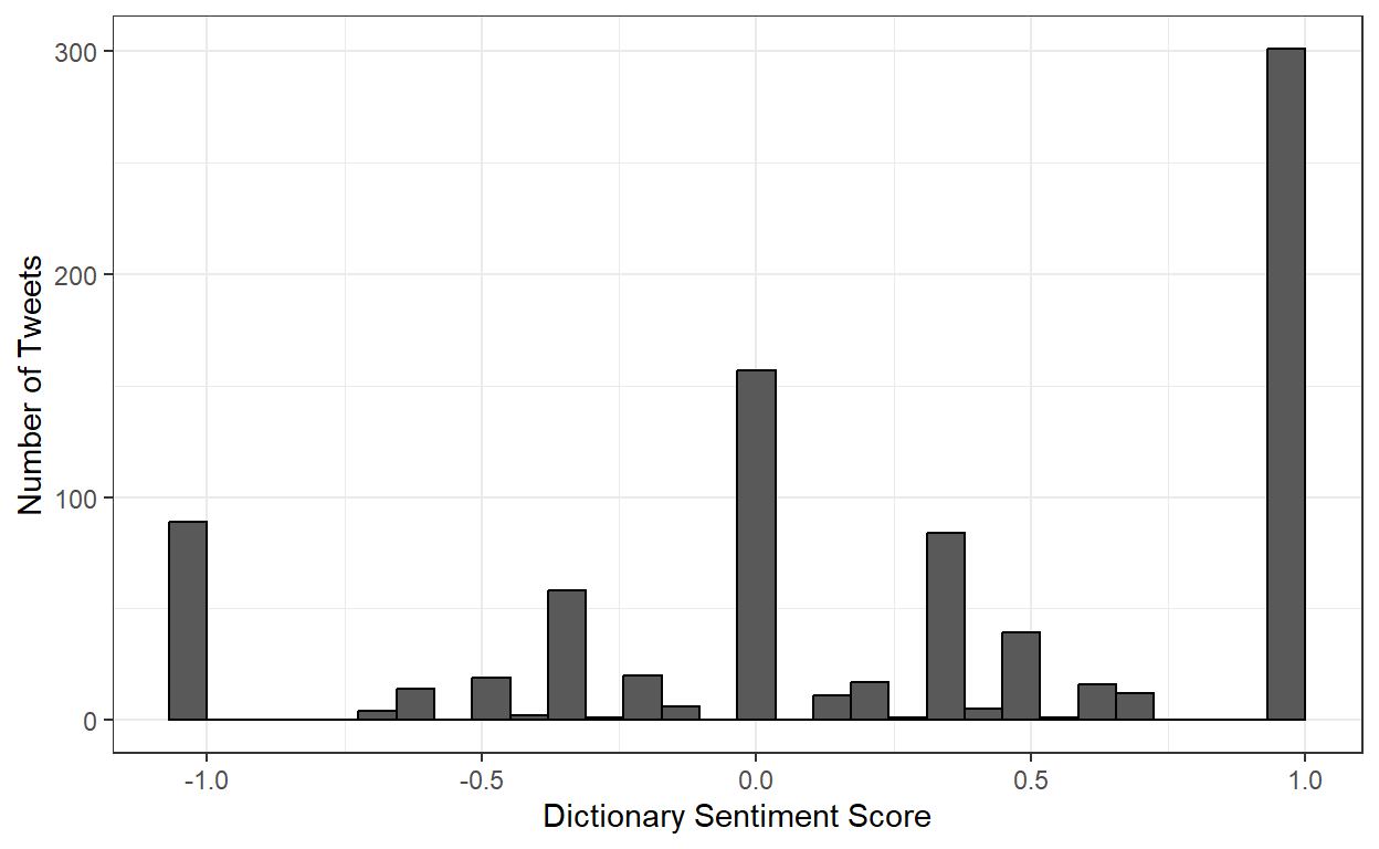
Looking at the histogram of results, it seems like the dictionary classifier is labeling a lot of these tweets as positive. A lot more than our expert coders did. What’s going on?
# find a tweet the experts coded as negative
# but the classifier coded as positive
tweets |>
  left_join(tidy_tweets, by = 'tweet_id') |>
  filter(expert1 == -1, expert2 == -1, expert3 == -1,
         sentiment_score == 1) |>
  pull(text) |>
  sample(3)
[1] "The NYS Supreme Court should hold their calendar and get Trump before Nov. That will make America great again. #TrumpTaxReturns \r\n#TrumpIsANationalDisgrace \r\n#TrumpMeltdown"
[2] "Thurgood Marshall’s successor on the Supreme Court was Clarence Thomas. I’ll never get over that."
[3] "If the supreme Court sides with Trump on his taxes we know it's all @senatemajldr doing for STACKING the court with bought and paid for judges like KAVANAUGH. We will have to increase pressure on @GOP up for re-election on their votes and hold them ACCOUNTABLE vote them all OUT"Ah. Well that’s embarrassing. Seems the bing lexicon codes the words “trump” and “supreme” as positive.
get_sentiments('bing') |>
  filter(word %in% c('trump','supreme'))
# A tibble: 2 × 2
word sentiment
<chr> <chr>
1 supreme positive
2 trump positive Perhaps this is an appropriate choice for the English language writ large, but for our specific corpus (tweets about Supreme Court cases during the Trump administration), it’s definitely inappropriate. Let’s see how the dictionary scores compare with the hand-coded scores.
tweets <- tweets |>
  left_join(tidy_tweets, by = 'tweet_id') |>
  mutate(expert_score = (expert1 + expert2 + expert3) / 3)

ggplot(data = tweets,
       mapping = aes(x = expert_score,
                       y = sentiment_score)) +
  geom_jitter(alpha = 0.5, width = 0.05) +
  theme_bw() +
  labs(x = 'Hand-Coded Sentiment',
       y = 'Dictionary Sentiment')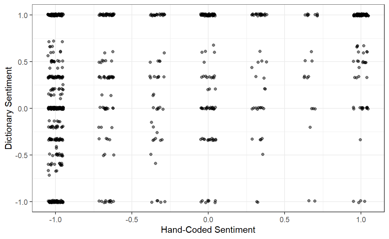
On the whole, it’s pretty bad (correlation = 0.333). When the tweets are genuinely positive, it seems that they contain a lot of positive words, so the dictionary method mostly gets it right. But when the tweets are negative, there may be a lot of sarcastic use of positive words, which trips up the classifier. For instance:
tweets |>
  filter(str_detect(text, 'sober')) |>
  pull(text)
[1] "I’m sure the news media will provide sober, nuanced analysis of Masterpiece Cake Shop. #SCOTUS"We want an approach that better predicts which words are most strongly associated with negative/positive sentiment in our particular corpus. For that we’ll need…
Supervised Learning
Both human coding and dictionary classification are examples of rule-based measurement. You decide in advance exactly what steps you will take to measure each document, and then you (or your computer) follow the rules you set out. The problem with such rules-based measures is that they are either:
- Not scalable (e.g. human-coding). For a dataset of 945 tweets, we were able to tackle it in relatively short order. But if we were interested in 100,000 tweets? Or a million tweets? There’s no way to scale that procedure, except with crowd coding on something like Amazon’s MTurk (Benoit et al. 2016; Carlson and Montgomery 2017), and that gets expensive quickly.
- Scalable, but terrible (e.g. dictionary methods). With rules-based classification, it’s trivial to classify a million tweets. But the results, as we have seen, are often crummy.
The best alternative to rules-based classification is statistical classification, and that is the topic of the page on supervised learning.
Practice Problems
- How accurate does the dictionary classifier need to be until it’s “good enough”? A useful benchmark is to compare your model against a null model. For example, in the Twitter corpus, how accurate is the null model “predict every tweet will be negative”?
- How accurate can you get the dictionary classifier to be, by varying the lexicon and modifying the word list to match our specific context (i.e. filtering out words whose dictionary meaning and context-specific meaning are different, like “Trump” and “Supreme”)?
Further Reading
- Silge & Robinson, Chapter 2
- Grimmer, Stewart & Roberts, Chapters 15-16
Yes, it was dreadful and I don’t recommend trying this at home.↩︎