At the end of the page on sentiment analysis, we lamented that hand-coding is too costly to scale, and rules-based classifiers are too inflexible to handle the subtleties of human language. On this page, we’ll demonstrate a different approach: take a corpus of pre-labeled documents, train a model to predict the labels, then use the predictions from that model to label other documents. This is called a supervised learning approach, and to illustrate, let’s replicate the exercise from Chapter 23 of Grimmer, Roberts, and Stewart (2022), predicting whether a set of tweets during the 2016 presidential election were written by Donald Trump or his campaign staff.
The Data
To start, let’s load the training data compiled by David Robinson.
library(tidyverse)
library(tidytext)
library(tidymodels)
library(lubridate)

load(url("http://varianceexplained.org/files/trump_tweets_df.rda"))

glimpse(trump_tweets_df)
Rows: 1,512
Columns: 16
$ text <chr> "My economic policy speech will be carried liv…
$ favorited <lgl> FALSE, FALSE, FALSE, FALSE, FALSE, FALSE, FALS…
$ favoriteCount <dbl> 9214, 6981, 15724, 19837, 34051, 29831, 19223,…
$ replyToSN <chr> NA, NA, NA, NA, NA, NA, NA, NA, NA, NA, NA, NA…
$ created <dttm> 2016-08-08 15:20:44, 2016-08-08 13:28:20, 201…
$ truncated <lgl> FALSE, FALSE, FALSE, FALSE, FALSE, FALSE, FALS…
$ replyToSID <lgl> NA, NA, NA, NA, NA, NA, NA, NA, NA, NA, NA, NA…
$ id <chr> "762669882571980801", "762641595439190016", "7…
$ replyToUID <chr> NA, NA, NA, NA, NA, NA, NA, NA, NA, NA, NA, NA…
$ statusSource <chr> "<a href=\"http://twitter.com/download/android…
$ screenName <chr> "realDonaldTrump", "realDonaldTrump", "realDon…
$ retweetCount <dbl> 3107, 2390, 6691, 6402, 11717, 9892, 5784, 793…
$ isRetweet <lgl> FALSE, FALSE, FALSE, FALSE, FALSE, FALSE, FALS…
$ retweeted <lgl> FALSE, FALSE, FALSE, FALSE, FALSE, FALSE, FALS…
$ longitude <chr> NA, NA, NA, NA, NA, NA, NA, NA, NA, NA, NA, NA…
$ latitude <chr> NA, NA, NA, NA, NA, NA, NA, NA, NA, NA, NA, NA…Throughout the 2016 presidential campaign, candidate Trump sent tweets from his personal Android phone, while staffers ghost-wrote tweets from an iPhone or web client. This provides us with the labels we need to build our model.
tweets <- trump_tweets_df |>
  select(.id = id,
         .source = statusSource,
         .text = text,
         .created = created) |>
  extract(.source, '.source', "Twitter for (.*?)<") |>
  filter(.source %in% c('iPhone', 'Android')) |>
  mutate(.source = factor(.source))

# (notice that I'm putting a dot in front of all these
# column names, on the off chance that words like "source"
# or "id" appear in the corpus after we tokenize)

tweets |>
  count(.source, hour = hour(with_tz(.created, "EST"))) |>
  mutate(percent = n / sum(n)) |>
  ggplot(aes(hour, percent, color = .source)) +
  geom_line() +
  scale_y_continuous(labels = percent_format()) +
  labs(x = "Hour of day (EST)",
       y = "% of tweets",
       color = "") +
  theme_minimal()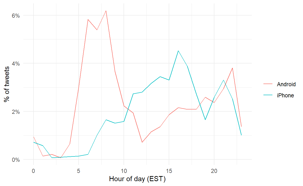
Trump is a very productive tweeter in the early morning and late evening. Next, let’s tokenize the tweets and convert into a document-term matrix. We’ll remove any stray HTML and rare words that only get used once or twice in the training set.
# pick the words to keep as predictors
words_to_keep <- tweets |>
  unnest_tokens(input = '.text',
                output = 'word') |>
  count(word) |>
  # remove numerals, URLs
  filter(str_detect(word, '.co|.com|.net|.edu|.gov|http', negate = TRUE)) |>
  filter(str_detect(word, '[0-9]', negate = TRUE)) |>
  # remove rare words
  filter(n > 2) |>
  pull(word)

# tokenize
tidy_tweets <- tweets |>
  unnest_tokens(input = '.text',
                output = 'word') |>
  filter(word %in% words_to_keep) |>
  count(.id, word) |>
  # compute term frequencies
  bind_tf_idf(term = 'word',
              document = '.id',
              n = 'n') |>
  select(.id, word, tf) |>
  # pivot wider into a document-term matrix
  pivot_wider(id_cols = '.id',
              names_from = 'word',
              values_from = 'tf',
              values_fill = 0)

# join with the training labels
tidy_tweets <- tweets |>
  select(.id, .source, .created) |>
  right_join(tidy_tweets, by = '.id')

dim(tidy_tweets)
[1] 1382 1156tidy_tweets[1:6, 1:5]# A tibble: 6 × 5
.id .source .created makeamericagreatagain of
<chr> <fct> <dttm> <dbl> <dbl>
1 7626698825… Android 2016-08-08 15:20:44 0 0
2 7626415954… iPhone 2016-08-08 13:28:20 0 0
3 7624396589… iPhone 2016-08-08 00:05:54 0 0
4 7624253718… Android 2016-08-07 23:09:08 0 0.0556
5 7624008698… Android 2016-08-07 21:31:46 0 0
6 7622845333… Android 2016-08-07 13:49:29 0 0.0476Underfitting and Overfitting
All supervised learning, in a nutshell, is an effort to find the sweet spot between a model that is too simple (underfitting) and one that is too complex (overfitting). With 1382 documents and 1153 possible predictors, there are an enormous number of possible models that we could fit.
To discipline ourselves, it is good practice to split the dataset into two parts: the training set, which we use to fit the model, and the test set, which we use to evaluate the predictions and see whether we did a good job.
tweet_split <- initial_split(tidy_tweets,
                             prop = 0.8)

train <- training(tweet_split)
test <- testing(tweet_split)
For our first stab at a model, consider what we remember about Trump’s tweeting style. Words and phrases that were distinctly Trump 2016, like “crooked”, “drain the swamp”, or “loser” might help predict whether it was him or a staffer doing the tweeting. Let’s fit a logistic regression including some of those keywords as predictors.
model1 <- logistic_reg() |>
  fit(formula = .source ~ crooked + dumb + emails +
        crowds + hillary + winning + weak,
      data = train)

tidy(model1)
# A tibble: 8 × 5
term estimate std.error statistic p.value
<chr> <dbl> <dbl> <dbl> <dbl>
1 (Intercept) -0.112 0.0646 -1.74 0.0820
2 crooked -10.6 5.61 -1.89 0.0587
3 dumb -341. 21260. -0.0160 0.987
4 emails 310. 31433. 0.00986 0.992
5 crowds -338. 20646. -0.0164 0.987
6 hillary -0.430 4.03 -0.107 0.915
7 winning 15.9 17.4 0.910 0.363
8 weak -382. 17063. -0.0224 0.982 This is a good start. Many of the words we chose are statistically significant predictors. But…
# out-of-sample fit
test |>
  bind_cols(predict(model1, test)) |>
  accuracy(truth = .source, estimate = .pred_class)
# A tibble: 1 × 3
.metric .estimator .estimate
<chr> <chr> <dbl>
1 accuracy binary 0.574test |>
bind_cols(predict(model1, test)) |>
conf_mat(truth = .source, estimate = .pred_class) |>
autoplot(type = 'heatmap')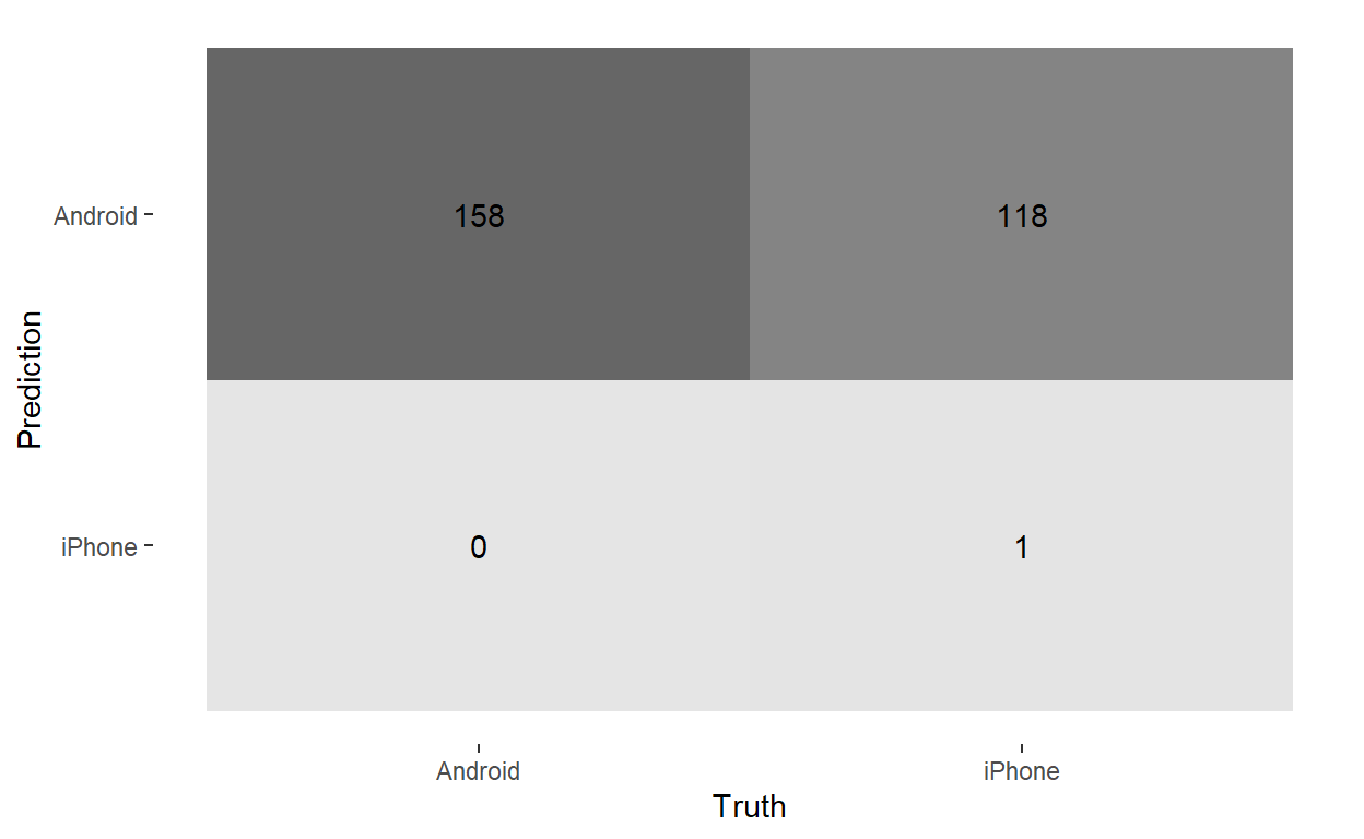
The model does a terrible job at out-of-sample prediction. Without a lot of information to go on (most of the tweets don’t contain one of those seven words) it predicts that every tweet but one was written by Trump. This is the hallmark of an underfit model: it doesn’t do any better than a null model that just predicts the most common class for every document.
What if we tried the opposite strategy, throwing every word into the model as a predictor? Would that perform better?
# overfit
model2 <- logistic_reg() |>
  fit(formula = .source ~ .,
      data = train |>
        select(-.id, -.created))

tidy(model2)
# A tibble: 1,154 × 5
term estimate std.error statistic p.value
<chr> <dbl> <dbl> <dbl> <dbl>
1 (Intercept) 3.90e15 428433735. 9094235. 0
2 makeamericagreatagain -8.86e13 429971626. -206105. 0
3 of -7.64e15 448759429. -17030047. 0
4 another -7.14e17 24267182028. -29417291. 0
5 best 2.09e17 12899282154. 16201657. 0
6 `for` -1.10e16 7083387182. -1555081. 0
7 golf -2.56e17 20103285575. -12727981. 0
8 great 2.22e16 784001592. 28323501. 0
9 highly 5.50e17 44774977456. 12278955. 0
10 thank 2.00e16 1292951204. 15481633. 0
# ℹ 1,144 more rows# in-sample fit
train |>
bind_cols(predict(model2, train)) |>
accuracy(truth = .source, estimate = .pred_class)# A tibble: 1 × 3
.metric .estimator .estimate
<chr> <chr> <dbl>
1 accuracy binary 0.995Clearly, this 1154 parameter model does a great job predicting the training set. But how is the prediction accuracy on the held-out test set?
# out-of-sample fit
test |>
  bind_cols(predict(model2, test)) |>
  accuracy(truth = .source, estimate = .pred_class)
# A tibble: 1 × 3
.metric .estimator .estimate
<chr> <chr> <dbl>
1 accuracy binary 0.527test |>
bind_cols(predict(model2, test)) |>
conf_mat(truth = .source, estimate = .pred_class) |>
autoplot(type = 'heatmap')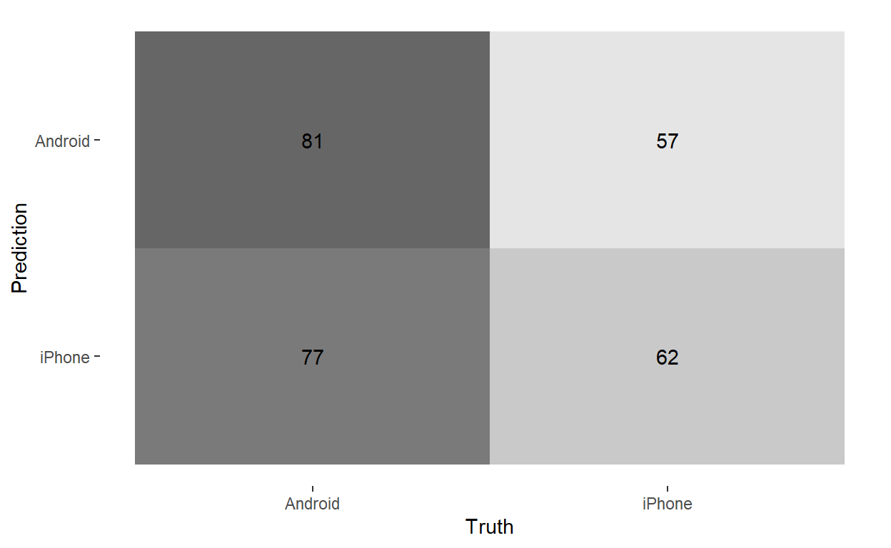
This is a hallmark of overfitting. The model is so complex that it is mistaking noise for signal, incorporating every random word that gets written by Trump of a staffer as a parameter estimate. For example, in the training set, there are 14 tweets that use the word “another”, 10 by Trump and the rest by staffers. The overfit model takes this as evidence that “another” is a Trumpy word. But that’s just a weird eccentricity of the training set; in the test set “another” is used more often by staffers. As a result, the overfit model actually performs worse out-of-sample than the underfit model.
While we want the model to do a good job minimizing prediction error in the training data, we also want to impose some constraint on how many words it can assign nonzero coefficients to. This is a job for regularization.
Regularization: Hitting the Sweet Spot
One way to impose a complexity constraint on our logistic regression model is with the LASSO. This approach estimates a set of coefficients that maximizes the likelihood of the data, subject to the constraint that \(\sum |\beta| < \frac{1}{\lambda}\). In other words, the sum total of the model’s coefficients can’t stray too far from zero. Let’s set that penalty term to 0.01 and see how we do.
# fit a regularized model (LASSO)
model3 <- logistic_reg(penalty = 0.01, mixture = 1) |>
  set_engine('glmnet') |>
  fit(formula = .source ~ .,
      data = train |>
        select(-.id, -.created))

tidy(model3)
# A tibble: 1,154 × 3
term estimate penalty
<chr> <dbl> <dbl>
1 (Intercept) 0.501 0.01
2 makeamericagreatagain 2.66 0.01
3 of 0 0.01
4 another 0 0.01
5 best 0 0.01
6 `for` 0 0.01
7 golf 0 0.01
8 great -0.527 0.01
9 highly 0 0.01
10 thank 9.84 0.01
# ℹ 1,144 more rows# in-sample fit
train |>
bind_cols(predict(model3, train)) |>
accuracy(truth = .source, estimate = .pred_class)# A tibble: 1 × 3
.metric .estimator .estimate
<chr> <chr> <dbl>
1 accuracy binary 0.944# out-of-sample fit
test |>
bind_cols(predict(model3, test)) |>
accuracy(truth = .source, estimate = .pred_class)# A tibble: 1 × 3
.metric .estimator .estimate
<chr> <chr> <dbl>
1 accuracy binary 0.798test |>
bind_cols(predict(model3, test)) |>
conf_mat(truth = .source, estimate = .pred_class) |>
autoplot(type = 'heatmap')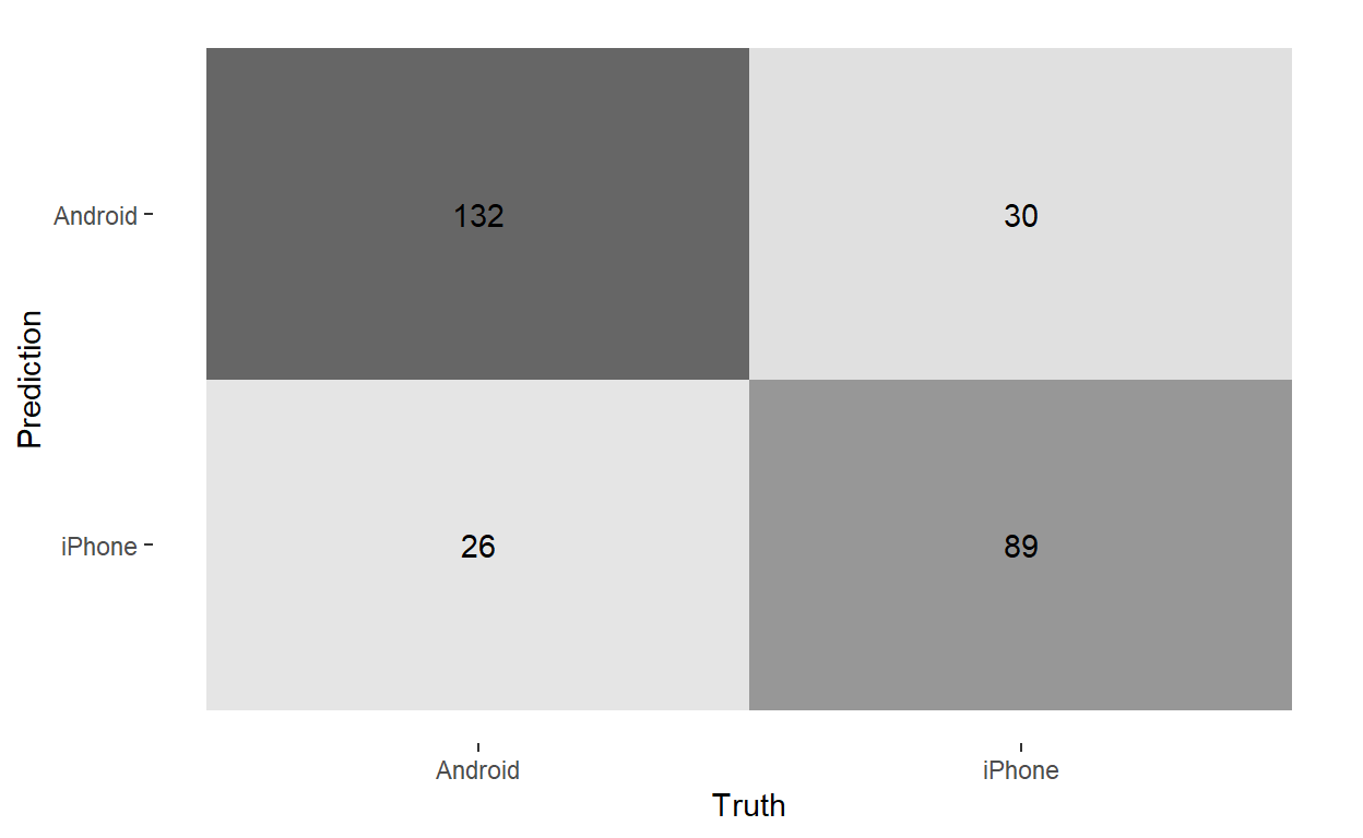
Regularization is powerful stuff. Not only does the regularized model perform much better out-of-sample than the first two models, but it gives us a set of 347 nonzero coefficients that we can interpret as the most strongly predictive words for whether a tweet was written by Trump or not.
tidy(model3) |>
  filter(estimate != 0) |>
  ggplot(mapping = aes(x = estimate,
                       y = fct_reorder(term, estimate))) +
  geom_col() +
  labs(x = 'Most Trumpy < - > Most Staffer-Speak',
       y = 'Term')
Practice Problems
Play around with the penalty hyperparameter until you find a better value for than 0.01. See the file
code/08_supervised-learning/predicting-trump-tweets-chap23.Rin the code repository for instructions more on tuning models through cross-validation with thetidymodelspackage.Fit a regularized logistic regression to predict whether the unattributed Federalist Papers were written by Hamilton or Madison, using the stop words document-term matrix we created earlier.
Further Reading
- David Robinson’s original post.
- Hvitfeldt & Silge (2022), particularly Chapter 7
- Grimmer, Stewart & Roberts, Chapters 17-19