Introduction to Political Methodology: Week 2

Reading

Teacup Giraffes: Mean, Median, and Mode
The Effect Chapter 3 (skip section 3.5 for now)

Optional Practice

The RStudio Primers are a set of helpful interactive data science tutorials from the people who brought you RStudio and the tidyverse. If you’re looking for additional practice, I recommend giving them a try!

Overview

This week, we introduce a tremendously fundamental concept in statistics, called the variable. What is a variable? Well, it’s a thing that varies across observations. Reason #1 why we’re using data to understand the world (i.e. a many story approach) is that it allows us to study variation – how things change from case to case.

In a tidy dataset, variables are the columns. For example, in the babynames dataset, the column named n contains the number of babies born in the United States in a given year with a given name and sex.

library(tidyverse)
library(babynames)

babynames

# A tibble: 1,924,665 × 5
    year sex   name          n   prop
   <dbl> <chr> <chr>     <int>  <dbl>
 1  1880 F     Mary       7065 0.0724
 2  1880 F     Anna       2604 0.0267
 3  1880 F     Emma       2003 0.0205
 4  1880 F     Elizabeth  1939 0.0199
 5  1880 F     Minnie     1746 0.0179
 6  1880 F     Margaret   1578 0.0162
 7  1880 F     Ida        1472 0.0151
 8  1880 F     Alice      1414 0.0145
 9  1880 F     Bertha     1320 0.0135
10  1880 F     Sarah      1288 0.0132
# ℹ 1,924,655 more rows

How do we make sense of all that information? The n column alone contains 1924665 numbers! Broadly speaking, there are two ways to do it: visualization and summarization.

Visualizing Distributions

The first way to make sense of all that data is to create a visual representation of the distribution, depicting how often different values occur.

# take the babynames dataset
babynames |> 
  # keep only babies born in the year 2000
  filter(year == 2000) |> 
  # pipe that dataset into a ggplot with the variable n on the x-axis
  ggplot(mapping = aes(x = n)) +
  # add a *histogram* geometry
  geom_histogram(color = 'black') +
  # make the x-axis a *logarithmic* scale
  scale_x_log10()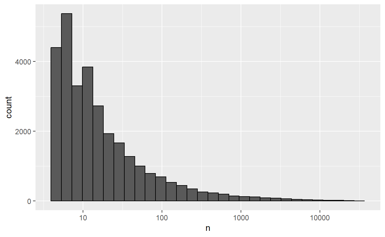

A few things to note here:

A histogram is a type of visualization where the height of each bar corresponds to the number of observations that fall into a certain range. I hope you agree that this is much more legible than looking through 1924665 numbers.
I plotted this histogram on a logarithmic scale, which means that each increment is a multiple of the previous increment (e.g. 10 is followed by 100, then 1,000, then 10,000).
This particular distribution is heavy tailed. There are thousands of names that appear less than a ten times, but only a handful of names that appear more than 10,000 times.

Summarizing Distributions

The second way to make sense of data is with statistics. A statistic is a number computed from data that summarizes or describes the distribution in some way.

For example, how many total babies were born in the United States in the year 2000?

babynames |> 
  filter(year == 2000) |> 
  summarize(total_babies = sum(n))

# A tibble: 1 × 1
  total_babies
         <int>
1      3778079

What was the median and mean value of n that year?

babynames |> 
  filter(year == 2000) |> 
  summarize(median_popularity = median(n),
            mean_popularity = mean(n))

# A tibble: 1 × 2
  median_popularity mean_popularity
              <int>           <dbl>
1                11            127.

Each of these summary statistics has a slightly different interpretation. The median tells us how many babies were born with the name in the exact middle of the popularity distribution that year. (In this case, there were 11 babies born with the name “Miraya”.) The interpretation of the mean is bit more complicated, but here’s a mental image I like. Imagine we took every baby born in the year 2000, sorted them by popularity of their name, and placed them on a massive see-saw. The mean is where you would place the fulcrum to exactly balance the babies on the left with the babies on the right. Because this distribution is so heavy tailed, that balance point is around 127.

Which is the right way to describe the distribution? Well, neither. They’re just different ways to describe the distribution, and we may want one or the other depending on what question we’re asking.

Using the group_by() function, we can compute summary statistics for different groups in the data.

babynames |> 
  filter(year == 2000) |> 
  group_by(sex) |> 
  summarize(median_popularity = median(n),
            mean_popularity = mean(n))

# A tibble: 2 × 3
  sex   median_popularity mean_popularity
  <chr>             <dbl>           <dbl>
1 F                    11            103.
2 M                    11            162.

Take a moment to ponder this result. What might it mean that the median for females and males is the same, but the mean for males is larger?

Problem Set

In our class folder, open RStudio with the project file intro-to-political-methodology.Rproj, then open problem-sets/problem-set-02.R.
In this problem set, we’ll summarize the distribution of survey respondents in the 2020 Cooperative Election Study (CES). First, what is the median age of respondents?
What is the median age of respondents who Strongly Approve of Trump’s performance as president? What’s the median age for each level of the trump_approval variable?
What’s the average age of people who watched TV news in the last 24 hours? Those who didn’t?
Are respondents who view religion as Very Important more or less likely to support a ban on assault rifles than those who view religion as Not Important At All?
See what else you can discover in the dataset, reporting at least three other summary statistics.
Compile the report to PDF (Ctrl + Shift + K) and submit the PDF at least 24 hours before our next class.